CDXWRF
CORDEX requirements of data for stake holders and decision making community, push the output of the atmospheric models, which demands that usually require time consuming post-process of the standard model output. In order to avoid this time and effort consuming post-processing task, here is presented the implementation of a new module into the Weather and Forecasting Model (WRF, Skamarok et al. 2008) module called module_diag_cordex with which is expected to substantially limit the need of post-processing.
PDF version of this page here Media:module_CORDEX_WRF.pdf
In order to get the code send an email to : lluis.fita [a] cima.fcen.uba.ar in order to keep a track and being able to inform of new versions/corrections.
Disclaimer
Authors decline any responsibility of the possible unexpected consequence of the use of this software. This piece
of code is provided following the scientific spirit of sharing knowledge and technical advances. Please, use it
with the same intention and willingness.
There are three working versions of the code for WRFV3.7.1, WRFV3.8.1, WRFV3.9.1.1, WRFV4.0. Different tests seem to show that the module slows model performance by a 40% (depending on namelist, compilation, ...)
Be aware that certain surface variables and their statistics (clWRF, Fita et al 2010) are retrieved from namelist configuration (from WRF users web page)
4. output_diagnostics = 1 in &time_control. Climate diagnostics. This option outputs 36 surface diagnostic variables:
maximum and minimum, times when max and min occur, mean value, standard deviation of the mean for T2, Q2, TSK, U10,
V10, 10 m wind speed, RAINCV, RAINNCV (the last two are time-step rain). The output goes to auxiliary output stream 3,
and hence it needs the following:

auxhist3_outname = “wrfxtrm_d<domain>_<date>”
auxhist3_interval = 1440, 1440,
frames_per_auxhist3 = 100, 100,
io_form_auxhist3 = 2
In this page CDXWRFevolution one founds updates, bug fixes of the module.
In this page CDXWRFversions one founds the different versions (tar.gz files) of the module.
With this module, now all CORDEX variables are available with the files wrfxtrm, wrfpress and wrfcdx, except for the fied values such as 'areacella'. See CDXvariablestable for more detail
CORDEX requirements
CORDEX requirements of data must cover all the possible needs of stake holders, and scientists working on the adaptation and mitigation strategies. They are grouped in different levels of frequency and priority. A working copy of this list is available here from the CORDEX convection permitting Flag Ship Pilot study.
Some of the variables are not directly computed in the WRF model which require to extend the model output in order to provide enough variables to post-process the variables.
The implementation of the module_diag_cordex module should allow to avoid the post-processing by computing the CORDEX-required (Core & Tier) variables during model integration. At the same time, some extra variables, which might be of interest to the community but not required by CORDEX, have also been added.
NOTE:
Be aware that any systematic checking process has been applied to this module. Use it and the
variables therein at your own risk !! It has been tested on a 2-nested domain configuration with the
inner domain at cloud resolving resolution (< 5 km, without cumulus scheme), making use of restarts
and on serial, pure distributed memory and hybrid distributed/shared parallel environment
module_diag_cordex
The module is basically based on two modules:
-
phys/module_diag_cordex.F: Main module which manages the calls to the variables and the accumulations for the means, ... -
phys/module_diagvar_cordex.F: Module with the computation of all the variables
This module is accompanied with a new Registry/registry.cordex where the variables and a new section
in the namelist.inpt labeled cordex are defined. There are other necessary complementary modifications on
phys/module_diagnostics_driver.F encompassed by the pre-compilaton flag CORDEXDIAG, as well some modifications in the main/depend.common and phys/Makefile.
Output is provided by the auxiliary history output #9 with a provisional file name: wrfcordex_d<domain>_<date>
All that variables which are only required at output time step, are computed only at that exact time.
Additional: pressure levels interpolation
At the same time, WRF can output on pressure levels while integration. However, initial version of the module does not include certain required CORDEX variables. The following ones have also been added to the code of the model and now they are also available:
-
wavertical wind speed [ms-1] -
husspecific humidity [1] -
uerEarth rotated x-compoment [ms-1] -
verEarth rotated y-compoment [ms-1] -
wswind speed [ms-1]
It has been accomplished after modifying the codes: Registry/registry.diags, phys/module_diagnostics_driver.F, phys/module_diag_pld.F and dyn_em/start_em.F. The three latest modifications are also encapsulated within precompilation flag CORDEXDIAG.
See more details in how to activate this option in WRF_users web-page over the namelist section diags&.
Additional: water budget
It has been added also the components of the atmospheric water budget. They are accumulated internally and vertically
integrated allover the column. In order to provide this capability, a series of modifications have been introduced in
dyn_em/solve_em.F
Installation
These steps must be followed prior the re-compilation of the WRF model and assuming that the process is started where the code resides (WRFV3). NOTE: make sure that the already compiled version of WRF and the version of the module are the same!
- Untar the file
$ tar xvfz WRFV[VERSION]_CORDEX.tar.gz
- It deflates all the required files and the modified orignal WRF files
main/depend.common
dyn_em/solve_em.F
dyn_em/start_em.F
phys/module_diagnostics_driver.F
phys/module_diag_cordex.F
phys/module_diagvar_cordex.F
phys/module_diag_pld.F
phys/Makefile
README.cordex
Registry/registry.cordex
Registry/registry.diags
- On the
Registry/Registry.EMadd the following line (after the last line with includeregistry.bdy_perturb(on WRFV3.7.1, WRFV3.8.1),registry.new3d_wif(on WRFV3.9.1.1))
include registry.cordex
- Clean the code (in order to avoid to run again configure one can make a copy of the
configure.wrfand recover it after the clean, otherwise it is erased)
$ cp configure.wrf configure.cordex.wrf
$ ./clean -a
$ cp configure.cordex.wrf configure.wrf
- edit the
`configure.wrf'and add the line (after the line-DNETCDFand/or–DCLWRFGHG)
-DCORDEXDIAG
- Set up (or not) the pre-compilation variable CDXWRF (after the line -DCORDEXDIAG)
-DCDXWRF=[value] \
- Accordingly to the value given to the pre-compilation variable
CDXWRFone obtains:- Without adding the variable: all CORDEX 'Core' variables
- CORDEX 'Tier1' variables: clivg, clivh, zmla, [cape/cin/zlfc/plfc/lidx]{min/max/mean}
- Accordingly to the value given to the pre-compilation variable
-DCDXWRF=1 \
- The same as with
CDXWRF=1and additional variables: ua, va, ws, ta, press, zg, hur, hus, tfog, fogvisbltymin, fogvisbltymax, fogvisbltymean, tdsmin, tdsmax, tdsmean and the Water-Budget relarted ones: wbacdiabh, wbacpw, wbacpw[c/r/s/i/g/h], wbacf, wbacf[c/r/s/i/g/h], wbacz, wbacz[c/r/s/i/g/h], wbacdiabh{l/m/h}, wbacpw{l/m/h}, wbacpw[c/r/s/i/g/h]{l/m/h}, wbacf{l/m/h}, wbacf[c/r/s/i/g/h]{l/m/h}, wbacz{l/m/h}, wbacz[c/r/s/i/g/h]{l/m/h}
- The same as with
-DCDXWRF=2 \
- Simultanesouly, one needs to modify the
Registry/registry.cordexaccordingly to the value ofCDXWRF:- Without adding
CDXWRF, nothing needs to be changed - Adding
CDXWRF=1, one needs to remove the comment##CDXWRF1##at the beginning of the line of the definition of certain variables - Adding
CDXWRF=2, one needs to remove the comment##CDXWRF1##and##CDXWRF2##at the beginning of the line of the definition of certain variables
- Without adding
- Additionally, one can also get the instantaneous values for the variables which only certain statistics (accumulation, minimum, mean, ...) are provided. In order to get them, one need to:
- Search in
phys/module_diagnostics_driver.Fandphys/module_diag_cordex.Fthe lines of code marked with'INSTVALS'and change accordingly. - Modify
Registry/registry.cordexaccordingly (removing##INST##at the beginning of the line of the definition of certain variables, and adding'h9'to certain others)
- Search in
- compile as always
$ ./compile em_real >& compile.log
Usage
These are the steps to use the module
- One need to add to the
'namelist.input'the auxiliar output number 9 (e.g. for output every 3 hours and 1-day files) at the`&history'section:
auxhist9_outname = "wrfcdx_d<domain>_<date>"
auxhist9_interval = 180, 180,
frames_per_auxhist9 = 8, 8,
io_form_auxhist9 = 2
- Also a new section should be added (assuming it will get complex and different implementations of the diagnostics might be necessary...) NOTE: do not copy directly this text. Fortran do not understand ':' as namelist input.
&cordex
 output_cordex      = 1
 psl_diag           = 1: sea-level pressure diagnostic following hydrostatic Shuell correction
                    = 2: psl diagnostic following a target pressure
                    = 3: psl diagnostic following ECMWF method (default)
 psmooth            = 5: passes of neighborgh filtering (3x3-grid point mean) of psfc for psl_diag=2
                      (default 5)
 ptarget            = 70000.: pressure [Pa] target to be used by psl_diag=2 (default 70000.)
 wsgs_diag          = 1: wind-gust diagnostic following Brasseur, 2001, MWR (default)
                    = 2: wsgs folllowing heavy precipitation method
 output_wb          = 1: whether water-budget variables have to computed (1) or not (0, default)
 wsz100_diag        = 1: wind extraoplation at z100m_wind using power-law method (default)
                    = 2: wind extraoplation at z100m_wind using logarithmic method
                    = 3: wind extraoplation at z100m_wind using Monin-Obukhov theory (NOT activated)
 z100m_wind         = 100.: height to extraplate winds (100. default)
 zmlagen_dqv        = 0.1: percentage of variation of mixing ratio to determine mixed layer depth used in
                        zmla computation (0.1 default)
 zmlagen_dtheta     = 1.5: increment in K of potantial temperature from its minimum within the MLD used in
                        zmla computation (1.5 default)
 potevp_diag        = 1: potential evapotranspiration following Penman-Monteith formulation after ORCHIDEE
                        implementation
 convxtrm_diag      = 0: diagnostic of extremes from convection indices: 0: No (default); 1: yes
 fogvisibility_diag = 1: diagnostic of visibility inside fog following Kunkel (1984)
                    = 2: RUC method (Smirnova et al., 2000)
                    = 3: FRAML 50% prob Gultepe and Milbrandt, (2010) (default)
 fogvars            = 1: variables to use to diagnose fog using 3D [hur] (default)
                    = 2: sfc [hus] (not available for Kunkel, 1984)
/
Pressure interpolation
Remember to activate section &diags in order to get pressure-level vertical interpolation of state variables (g.e.: assuming 6 levels only and output every 3 hours)
&time_control
(...)
auxhist23_outname="wrfpress_d<domain>_<date>"
io_form_auxhist23 = 2,
auxhist23_interval = 180, 180,
frames_per_auxhist23 = 100, 100,
(...)
/

(...)

&diags
p_lev_diags = 1,
num_press_levels = 6,
press_levels = 100000, 92500, 85000, 70000, 50000, 20000
use_tot_or_hyd_p = 1
p_lev_missing = -999.
/
Variables
These are the different variables added and their implementations from the WRF point of view. There might be necessary to revise some of them, or even decide which version to use In case of accumulation/mean they are also be included
These variables are:
- Instantaneous diagnostics (only computed on output times)
- Core
- -
prw:Total water path - -
clwvi:Total liquid water path (QCLOUD + QRAIN) - -
clivi:Total ice water path (QSNOW+QICE+GRAUPEL+QHAIL) - -
uas:10m earth-rotated eastward wind [ms-1] - -
vas:10m earth-rotated northward wind [ms-1] - -
wss:10m wind speed [ms-1] - -
hurs:2m relative humidty [1] - -
huss:2m specific humidty [1] - -
mrso:total soil moisture content [kgm-2] - -
slw:total liquid water content [kgm-2] - -
ws100:100m wind speed [ms-1] - -
uz100:100m wind x-direction [ms-1] - -
vz100:100m wind y-direction [ms-1] - -
tauu, tauuv:components of the downward wind stress at 10 m [m2s-2] (might be zero if sf_sfclay_physics /= 1, 5) - -
tauugen, tauuvgen:generic components of the downward wind stress at 10 m [m2s-2] - -
cdcdx:drag coefficient [-] (might be zero if sf_sfclay_physics /= 1, 5) - -
cdgen:generic drag coefficient [-] - -
ps:surface pressure [Pa] - -
ts:skin temperature [K]
- Tier1
- -
zmla:pbl height following a generic method [m] - -
clgvi:Total graupel path (QGRAUPEL) - -
clhvi:Total hail path (QHAIL)
- Additional
- -
ua:3D earth-rotated eastward wind [ms-1] - -
va:3D earth-rotated northward wind [ms-1] - -
ws:3D wind speed [ms-1] - -
ta:3D air-temperature [K] - -
press:3D air pressure [Pa] - -
zg:3D geopotential height [m] - -
hur:3D relative humidty [1] - -
hus:3D specific humidty [1] - -
psl:sea level pressure [Pa] (three different ways)
- Only via changes in the registry
- -
clt:total cloud cover [1] - -
cll:low-level cloud cover [1] - -
clm:mid-level cloud cover [1] - -
clh:high-level cloud cover [1] - -
cape:Convective Available Potential Energy [Jkg-1] - -
cin:Convective inhibition [Jkg-1] - -
zlfc:Height at the Level of free convection [m] - -
plfc:Pressure at the Level of free convection [Pa] - -
li:Lifted index [1] - -
tds:2m dew point temperature [K]
- Accumulated or similar time dependency (computed at every time-step). They are initialized after each output time-step. Thus, they represent statistics (mean, accumulation) only from between output time-steps.
- Core
- -
cltmean:mean clt - -
cllmean:mean cll - -
clmmean:mean clm - -
clhmean:mean clh - -
wsgsmax:maximum surface wind gust [ms-1] (two different methods) - -
ugsmax:eastward maximum surface gust wind direction [ms-1] - -
vgsmax:northward maximum surface gust wind direction [ms-1] - -
wsgspercen:percentage of times when grid point got gust wind [%] - -
totwsgsmax:maximum surface wind gust [ms-1] (addition of different methods) - -
totugsmax:eastward maximum surface gust wind direction [ms-1] - -
totvgsmax:northward maximum surface gust wind direction [ms-1] - -
totwsgspercen:percentage of times when grid point got total gust wind [%] - -
wsz100max:maximum 100m wind [ms-1] (two different methods) - -
uz100max:eastward maximum 100m wind direction [ms-1] - -
vz100max:northward maximum 100m wind direction [ms-1] - -
sund:sunshine length [s] - -
rsds:mean surface Downwelling Shortwave Radiation [Wm-2] - -
rlds:mean surface Downwelling Longwave Radiation [Wm-2] - -
hfls:mean surface Upward Latent Heat Flux [Wm-2] - -
hfss:mean surface Upward Sensible Heat Flux [Wm-2] - -
rsus:mean surface Upwelling Shortwave Radiation [Wm-2] - -
rlus:mean surface Upwelling Longwave Radiation [Wm-2] - -
rsusgen:mean generic surface Upwelling Shortwave Radiation [Wm-2] - -
rlusgen:mean generic surface Upwelling Longwave Radiation [Wm-2] - -
evspsbl:mean evaporation [kgm-2s-1] - -
evspsblpot:mean potential evapotranspiration [kgm-2s-1] - -
evspsblpotgen:mean generic potential evapotranspiration [kgm-2s-1] - -
snc:mean snow area fraction [%] - -
snd:mean snow depth [m] - -
mrros:mean surface Runoff [kgm-2s-1] - -
mrro:mean total Runoff [kgm-2s-1] - -
mrsol:mean total water content of soil layer [kgm-2] - -
pr:precipitation flux [kgm-2s-1] - -
prl:large scale precipitation flux [kgm-2s-1] - -
prc:convective precipitation flux [kgm-2s-1] - -
prsh:shallow-cumulus precipitation flux [kgm-2s-1] - -
prsn:solid precipitation flux [kgm-2s-1] - -
snw:accumulated snow [ksm-2] - -
rsdt:Top Of the Atmosphere incident shortwave radiation [kgm-2] - -
rsut:TOA outgoing shortwave radiation [kgm-2] - -
rlut:TOA outgoing Longwave radiation [kgm-2]
- Tier1
- -
capemin:minimum CAPE [Jkg-1] (activated if convxtrm_diag =1) - -
cinmin:minimum CIN [Jkg-1] (activated if convxtrm_diag =1) - -
zlfcmin:minimum height at LFC [m] (activated if convxtrm_diag =1) - -
plfcmin:minimum Pressure at LFC [Pa] (activated if convxtrm_diag =1) - -
lidxmin:minimum Lifted index [1] (activated if convxtrm_diag =1) - -
capemax:maximum CAPE [Jkg-1] (activated if convxtrm_diag =1) - -
cinmax:maximum CIN [Jkg-1] (activated if convxtrm_diag =1) - -
zlfcmax:maximum height at LFC [m] (activated if convxtrm_diag =1) - -
plfcmax:maximum Pressure at LFC [Pa] (activated if convxtrm_diag =1) - -
lidxmax:maximum Lifted index [1] (activated if convxtrm_diag =1) - -
capemean:mean CAPE [Jkg-1] (activated if convxtrm_diag =1) - -
cinmean:mean CIN [Jkg-1] (activated if convxtrm_diag =1) - -
zlfcmean:mean height at LFC [m] (activated if convxtrm_diag =1) - -
plfcmean:mean Pressure at LFC [Pa] (activated if convxtrm_diag =1) - -
lidxmean:mean Lifted index [1] (activated if convxtrm_diag =1)
- Additional (not required by CORDEX)
- -
tfog:time of presence of fog [s] - -
fogvisbltymin:minimun visibility inside fog [km] - -
fogvisbltymax:maximun visibility inside fog [km] - -
fogvisbltymean:mean visibility inside fog [km] - -
tdsmin:minimum 2m dew point temperature [K] - -
tdsmax:maximum 2m dew point temperature [K] - -
tdsmean:mean 2m dew point temperature [K]
- Additionally added referred to the water budget in the atmosphere:
-
wbacdiabh:Water-budget vertically integrated accumulated of diabatic heating from microphysics [K] -
wbacpw, wbacpw[c/r/s/i/g/h]:Water-budget vertically integrated accumulated total tendency for water vapour, cloud, rain, snow, ice, graupel, hail [mm] -
wbacf, wbacf[c/r/s/i/g/h]:Water-budget vertically integrated accumulated horizontal advection for water vapour, cloud, rain, snow, ice, graupel, hail [mm] -
wbacz, wbacz[c/r/s/i/g/h]:Water-budget vertically integrated accumulated vertical advection for water vapour, cloud, rain, snow, ice, graupel, hail [mm] -
wbacdiabh{l/m/h}:Water-budget vertically integrated accumulated of diabatic heating from microphysics at low, medium and high levels (same as cloudiness) [K] -
wbacpw{l/m/h}[v/c/r/s/i/g/h]:Water-budget vertically integrated accumulated total tendency for water vapour, cloud, rain, snow, ice, graupel, hail at low, medium and high levels (same as cloudiness) [mm] -
wbacf{l/m/h}[v/c/r/s/i/g/h]:Water-budget vertically integrated accumulated horizontal advection for water vapour, cloud, rain, snow, ice, graupel, hail at low, medium and high levels (same as cloudiness) [mm] -
wbacz{l/m/h}[v/c/r/s/i/g/h]:Water-budget vertically integrated accumulated vertical advection for water vapour, cloud, rain, snow, ice, graupel, hail at low, medium and high levels (same as cloudiness) [mm]
-
- Pressure interplation (Core)
- -
hus_pl:specific humidity [1] - -
w_pl:vertical wind speed [ms-1] - -
uer_pl:Earth-rotated wind x-component [ms-1] - -
ver_pl:Earth-rotated wind y-component [ms-1] - -
ws_pl:wind speed [ms-1]
- -
clt: total cloudiness
This variable computes the total cloudiness above a grid point taking as input the cloud fraction of a given grid cell and level.
NOTE:
cloud fraction in WRF is computed by the radiative scheme, which is called at a frequency given by radt.
It should be taking into account when one gets any accumulation of any value retrieved from it. Otherwise,
one could compute the cloud fraction at every time-step (using any of the subroutines from
module_radiation_driver.F: cal_cldfra1, cal_cldfra2, cal_cldfra3), but then it will not be consistent in
what was already considered whilst model integration
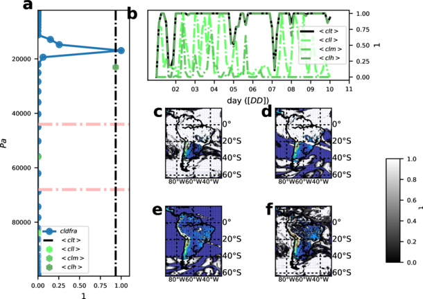
The most common implementation of ‘clt’ found in different other models assumes ‘random overlapping’ and its implemented in most of the global climate models. Here the methodology from the GCM (LMDZ, Hourdin et al., 2006) was implemented. In this GCM, calculation of the total cloudiness is done inside the subroutine newmicro.f90.
cllmh: low, medium and high cloudiness
This variable computes the total cloudiness above a grid point at different vertical intervals (low: p ≥ 680hP a, medium: 680 < p ≥ 400 hP a, high: p < 400 HP a) taking as input the cloud fraction of a given grid cell.
As in the case of the ‘clt’ calculation from LMDZ has already been implemented as an independent subroutine. See in figure 1 the result of the implementation
wsgsmax: Maximum Near-Surface Wind Speed of Gust
The wind gust accounts for the wind from upper levels that is projected to the surface due to instability within the boundary layer. It can have different implementations. Winds are Earth-rotated.
-
Brasseur01:An implementation of a wind gust following Turbuelent Kinetic Energy (TKE) estimates and stability by virtual temperature (θv , see mainly equation 1) reproducing Brasseur (2001) from the clWRF (clWRF Fita et al., 2010) [wsgs_diag = 1]
-
WRF_afwa_diagnostics:Inside the WRF modulemodule_diag_afwa.Fthere is an implementation of the calculation of the wind gust which only occurrs as a blending of upper-level winds (around 1km above ground zagl; -1 zagl(k1000 ) ≥ 1000 m, see equation 2) above a given maximum precipitation inrensity of pratemm_hr ≥ 50 mm [wsgs_diag = 2]
These two methodologies have been implemented and can be switched by a new namelist.input parameter labeled wsgs_diag (in cordex section). Its default value is 1 It comes out, that both methodologies provide wind gust estimation (WGE) from two different perspectives: mechanic and convective. In order to take into account both winds gusts, another variable as the addition of both estimations is provided as totwsgsmax, totugsmax, totvgsmax, totwsgspercen. On figure 2 is shown the different outcomes applying each approximation
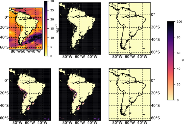
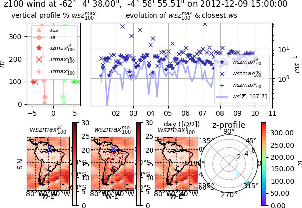
wsgsmax100: Daily Maximum Near-Surface Wind Speed of Gust at 100 m
The wind gust at 100 m is understood that should follow a similar implementation than for the wsgsmax, but at 100 m, an extrapolation of such turbulent phenomena it would require a complete new set of equations which have not yet been placed.
Instead as a way to overcome it, the estimation of maximum wind speed at 100 m is provided. Provided winds are also Earth-rotated. After PhD thesis of Jourdier (2015), two different methodologies are implemented to estimate the wind at 100 m above ground:
- Following power-law wind vertical distribution, as it is depicted in equation 3 using the upper-level atmospheric wind speed below (k100) and above (k100) the height above ground of 100 m (zagl) [wsz100_diag = 1]
- Following logarithmic-law wind vertical distribution, as it is depicted in equation 4 using upper-level atmospheric wind speed below (k100) and above (k100) the height above ground of 100 m (zagl) [wsz100_diag = 2]
- Following Monin-Obukhov theory is implemented and was tested, but it is not useful for heights larger than few decameters (z > 80. m). However, the necessary code to extrapolate the wind at given height is left commented just in case someone wants to use it.
These two methodologies have been implemented and can be switched by a new namelist.input parameter labeled wsz100_diag (in cordex section). Its default value is 1. Even one can select another height for the estimation by providing the new parameter z100m_wind with a different value than 100 m (default value)
On figure 3 is shown the different outcomes applying each approximation. There are some problems on MoninObukhov application under certain stable conditions (too small Obukhov length)
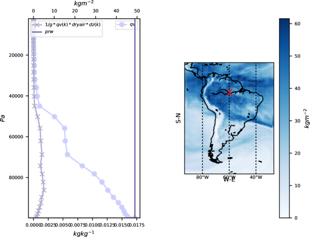
prw: precipitable water or water vapor path
This variable accounts for the column integrated amount of water vapor.
This one is already implemented in a old WRF tool for vertical interpolation called p_interp.F related to the clWRF. The general equation following WRF standard variables as:
where mu: perturbation dry air mass in column (Pa), mub: base-state dry air mass in column (Pa), g: gravity (ms-2), e_vert: total number of vertical levels, qvapor: mixing ratio of water vapour (kgkg-1), dnw: full-sigma eta-layer height. See an example on figure 4
clwvi: condensed water path
This variable provides similar information, but for the liquid condensed water species. It is the same calculation as in 5, but replacing QVAPOR by QCLOUD + QRAIN
clivi: ice water path
This variable provides similar information, but for the liquid condensed water species. It is the same calculation as in 5, but replacing QVAPOR by QICE + QSNOW + QGRAUPEL + QHAIL
clgvi: graupel water path
This variable provides similar information, but for the liquid condensed water species. It is the same calculation as in 5, but replacing QVAPOR by QGRAUPEL. This variable is part of the ‘Tier1’ level and it is only accessible if pre-compilation variable CDXWRF is set to 1. See section [3] for more detail.
clhvi: hail water path
This variable provides similar information, but for the liquid condensed water species. It is the same calculation as in 5, but replacing QVAPOR by QHAIL. This variable is part of the ‘Tier1’ level and it is only accessible if pre-compilation variable CDXWRF is set to 1. See section [3] for more detail.
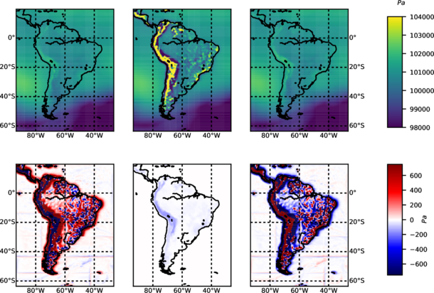
psl: sea level pressure
This accounts for the pressure at the sea level (extrapolation of the pressure at the level of the sea). That means the pressure that might be without the presence of orography. Three different methodologies have been implemented
- One using hydrostatic-Shuell method already implemented in the the module
phys/module_diag_afwa.F(assuming a constant lapse-rate of 6.5 K km-1) [psl_diag = 1] - Using smoothed surface pressure and a target upper-level pressure, already implemented in
p_interp.F90[psl_diag = 2] - ECMWF method taken from LMDZ from the module pppmer.F90, following the methodology by Mats Hamrud and Philippe Courtier from ECMWF [psl_diag = 3]
These three methodologies have been implemented and can be switched by a new namelist.input parameter labeled psl_diag (in cordex section). Its default value is 3. Even, on using the 'ptarget' method (psl_diag = 2) one can select the degree of smoothing of the surface place by the selecting the number of times that the smoothing (as the mean of the point and its surrounding 8 neighbors) has to be applied (psmooth, default 5) and the upper pressure to be used as target (ptarget, default 70000 Pa).
On figure 5 is shown the different outcomes applying each approximation. There are some problems with the ptarget methodology in both psl estimate and borders for each parallel process on applying the smoothing
cape: convective available potential energy
This variable accounts for all the energy that convectively might be released. From AMS glossary is described as: (CAPE)
"On a thermodynamic diagram this is called positive area and can be seen as the region between the lifted parcel process curve and the environmental sounding, from the parcel’s level of free convection to its level of neutral buoyancy. CAPE may be expressed as follows:
![]()
where Tvp is the virtual temperature of a lifted parcel moving upward moist adiabatically from the level of free convection to the level of neutral buoyancy, Tve is the virtual temperature of the environment, Rd is the specific gas constant for dry air, pf is the pressure at the level of free convection, and pn is the pressure at the level of neutral buoyancy. The value depends on whether the moist-adiabatic process is considered to be reversible or irreversible (conventionally irreversible, or a pseudoadiabatic process in which condensed water immediately falls out of the parcel) and whether the latent heat of freezing is considered (conventionally not). It is assumed that the environment is in hydrostatic balance and that the pressure of the parcel is the same as that of the environment. Virtual temperature is used for the parcel and environment to account for the effect of moisture on air density."
At this version of the module, only one implementation of the variable has been implemented. WRF model already provides a way of calculation of the variables inside the module phys/module_diag_afwa.F (sinve WRF version V3.6) via the function Buoyancy, which at the same time it provides: Convective inhibition (CIN), Height at the Level of free convection (ZLFC), Pressure at the Level of free convection (PLFC) and Lifted index (LI). Tacking advantage of this, these extra four variables are also provided. This vertical integrated diagnostics have a high computational cost. In order to minimize it, by default, they are only computed at output time-step. However, if user requires Tier1 variables which are related to the statistics of these diagnostics: capemin, capemax, capemean, cinmin, cinmax, cinmean, zlfcmin, zlfcmax, zlfcmean, plfcmin, plfcmax, plfcmean, limin, limax and limean, then these diagnostics are computed at all time-steps. This behavior of the module is regulated via the namelist parameter convxtrm_diag (defaul value is 0, meaning no computation), and setting the pre-compilation flag CDXWRF to 1 and perform some complementary modifications in module's Registry file Registry/registry.cordex. See section [3] for more detail.
cin: convective inhibition
This variable accounts for the process which inhibits the convection. Already provided by the implementation of the AFWA’s CAPE calculation From AMS glossary is described as: CIN) "The energy needed to lift an air parcel upward adiabatically to the lifting condensation level (LCL) and then as a psuedoadiabatic process from the LCL to its level of free convection (LF C). For an air parcel possessing positive CAP E, the CIN represents the negative area on a thermodynamic diagram. The negative area typically arises from the presence of a lid, or the amount of kinetic energy that must be added to a parcel to enable that parcel to reach the LF C. Even though other factors may be favorable for development of convection, if convective inhibition is sufficiently large, deep convection will not form. The convective inhibition is expressed (analogously to CAPE) as follows:
where pi is the pressure at the level at which the parcel originates, pf is the pressure at the LFC, Rd is the specific gas constant for dry air, Tvp is the virtual temperature of the lifted parcel, and Tve is the virtual temperature of the environment. It is assumed that the environment is in hydrostatic balance and that the pressure of the parcel is the same as that of the environment. Virtual temperature is used for the parcel and environment to account for the effect of moisture on air density."
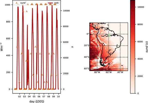
sund: duration of sunshine
This variable accounts for the time where short-wave radiation is above 120 Wm-2
See results of the variable in figure 6
hur: relative humidity
3D atmospheric relative humidity on standard model η levels can be obtained following the Clausius-Clapeyron formula and its approximation from the well-known August-Roche-Magnus formula of saturated water vapor pressure es. This is an 'additional' variable which requires setting the pre-compilation flag CDXWRF to 2 and perform some complementary modifications in module's Registry file registry.cordex. See section [3] for more detail.
being tempC: temperature (◦C), presshPa: pressure (hPa), es: saturated water vapor pressure (Pa), ws: saturated mixing ratio (kgkg-1), q: mixing ratio (kgkg-1).
hus: specific humidity
3D atmospheric specific humidity (From the AMS glossary hus) on standard model η levels is computed according to equation 11. This is an 'additional' variable which requires setting the pre-compilation flag CDXWRF to 2 and perform some complementary modifications in module's Registry file Registry/registry.cordex. See section [3] for more detail.
where rv: mixing ratio (kgkg-1)
zg: geopotential height
This variable states for the 3D atmospheric geopotential height on standard model η levels. WRF model integrates the perturbation of the geopotential field from a reference or base one. Thus to obtain the full geopotential height is required to combine two different fields as it is shown in equation 12. This is an 'additional' variable which requires setting the pre-compilation flag CDXWRF to 2 and perform some complementary modifications in module’s Registry file Registry/registry.cordex. See section [3] for more detail.
where PHB, WRF base geopotential height (m2s-2), PH, WRF perturbation geopotential height (m2s-2)
press: air-pressure
This variable states for the 3D atmospheric pressure on standard model η levels. WRF model integrates the perturbation of the pressure field from a reference one. thus to obtain the full pressure is required to combine two different fields as it is shown in equation 13. This is an 'additional' variable which requires setting the pre-compilation flag CDXWRF to 2 and perform some complementary modifications in module's Registry file Registry/registry.cordex. See section [3] for more detail.
where PB, WRF base pressure (Pa), P, WRF perturbation pressure (Pa)
ta: air-temperature
This variable states for the 3D atmospheric temperature on standard model η levels. WRF model equations are based on potential temperature. Thus a conversion to actual temperature is required and it is performed as it is shown in equation 14. This is an 'additional' variable which requires setting the pre-compilation flag CDXWRF to 2 and perform some complementary modifications in module's Registry file Registry/registry.cordex. See section [3] for more detail.
where T, WRF temperature (K, which is as potential temperature), PB, WRF base pressure (Pa), P, WRF perturbation pressure (Pa), p0: pressure reference 100000 (Pa)
ua/va: air-wind Earth oriented
This variable states for the 3D atmospheric wind speed following Earth coordinates on standard model η-levels. WRF model equations use stagger winds following grid direction. In order to get actual winds following Earth geographical coordinates, a transformation shown in equation 15 is required. This is an ‘additional’ variable which requires setting the pre-compilation flag CDXWRF to 2 and perform some complementary modifications in module's Registry file Registry/registry.cordex. See section [3] for more detail.
where Ustg: x-staggered WRF eastward wind (ms-1), Vstg: y-staggered WRF northward wind (ms -1), Uunstg: unstaggered WRF eastward wind (ms-1), Vunstg: unstaggered WRF northward wind (ms-1), cosa: local cosine of map rotation (1), sina: local sine of map rotation (1).
tauuv
Surface Downdward wind stress at 10m. This variable account for the force that winds exercises to the surface. It is implemented following the equation 16, begin CD drag coefficient. Winds are Earth-rotated.
where, CD: drag coefficient (1) which in WRF is non-zero only for certain options of surface layer physics if sf_sfclay_physics /= 1, 5 (1: MM5-similarity, 5: MYNN surface layer), uas: eastward 10 m surface wind (ms-1), vas: northward 10 m surface wind (ms-1)
evspsblpot
This variable accounts for theoretical maximum evaporation that is possible to occur. Potential evapotranspiration is computed following its computation from [ORCHIDEE] model (Organising Carbon and Hydrology In Dynamic Ecosystems. The implementation is retrieved from the module src_sechiba/enerbil.f90 and basically consists on an implementation of the Penman-Monteith formulation (Monteith, 1965). It is a simple formulation (see equation 16)
where qc: surface drag coefficient (ms-1), q2sat: Saturated air at 2m (kgkg-1, using August-Roche-Magnus approximation and assuming to be q2 &SIM; qsfc), uas,vas: 10 m wind components ms-1), CD: Drag coefficient (-, only available for surface layer schemes MM5-similarity and MYNN)
Up to now there is only one implementation and it is selected via namelist parameter potevap_diag, up to now only with value 1 for the ORCHIDEE implementation
rsus
Surface Upwelling Shortwave Radiation, is understood as the shortwave radiation from land. It is provided accumulated by radiation schemes CAM and RRTMG (sw_ra_scheme = 3,4) in variable SWUPB.
rlus
Surface Upwelling Longwave Radiation, is understood as the longwave radiation from land. It is provided accumulated by radiation schemes CAM and RRTMG (sw_ra_scheme = 3,4) in variable SLUPB.
pr
Total precipitation flux is computed as the sum of all the types of precipitation as it is shown in equation 18
where prc: convective precipitation (kgm-2), prl: large-scale precipitation (kgm-2), prsh: shallow-cumulus precipitation (kgm-2), Nsteps: number of time steps and δt: time-step length (s).
prsn
Solid precipitation flux accounts for all the precipitation which is frozen. Depending on the micro-physics scheme it might account for the precipitation of: snow, graupel and hail. It is computed as it is shown in equation 19
where pr: total precipitation (kgm-2), sr: fraction of solid precipitation (1, variable included in WRF), Nsteps: number of time steps and δt: time-step length (s)
Generic variables
Some of the diagnostics required by CORDEX depend on the approximations, equations, methodologies and observations used to compute them. This make model intercomparison exercises very difficult because values might differ from one implementation to another one. In a way to overcome this issue, a series of variables are also provided in a 'generic' form (when possible) meaning that they are obtained directly from well established variables. Thus, these generic form of the diagnostics become 'independent' of model's implementation.
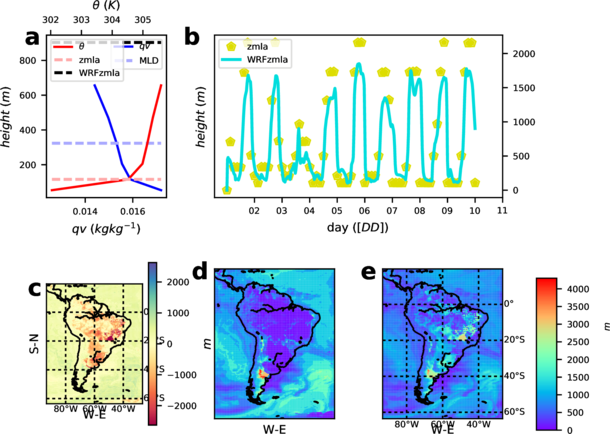
zmlagen: generic boundary layer height
Boundary layer height is a clear example of model dependence and even scheme dependence of how a diagnostic is computed. Each pbl scheme has its own assumptions and has to be compiled in a specific way. This variable is provided with the 'Tier1' level of variables and requires to set the pre-compilation flag CDXWRF to 1 and perform some complementary modifications in module's Registry file Registry/registry.cordex</CORDEX>. See section [3] for more details.
Pursuing this goal, we implemented a general definition for the boundary layer height as it was done in (García-Díez et al., 2013) after (Nielsen-Gammon et al., 2008). The method consists in defining the height of the boundary layer as the first level where potential temperature exceeds the minimum potential temperature reached in the mixed layer (ML) by more than 1.5 K. It has been implemented as it is shown below:
- Mixed layer depth (kMLD) first layer at which the variation of mixing ratio upwards from first layer value achieves a given percentage:
 > δqv (here applied a δqv = 0.1)
- Minimum potential temperature within the MLD: θminM LD = min(θ(1), ..., θ(kM LD ))
- Boundary layer level (kzmla ) first level where: θ(kzmla ) + δθ > θminM LD (here δθ = 1.5 K)
- Boundary layer height (zmla) height above ground (zagl): zmla = zagl(kzmla )
Comparison of this implementation with the zmla directly provided by WRF’s pbl scheme is shown in figure 14.
No general rule has been applied to determine the correct value of δqv used to determine depth of mixed layer. They can be determined by the <CODE>namelist.input parameters zmlagen_dqv for δqv (default value 0.1) and zmlagen_dtheta for δθ (default value 1.5 K)
cdgen
Drag coefficient at surface. Computation of drag coefficient depends on selected surface scheme. In order to avoid this scheme dependency, a general calculation of the coefficient has been introduced as it is shown in equation 20, after Garratt (1992).
Being, u∗: from similarity theory (ms-1), wss: 10 m wind speed (ms-1)
tauuvgen: generic surface downdward wind stress
Generic surface downdward wind stress at 10m. It is implemented following the equation 21. Winds are Earth-rotated.
where CDgen generic drag coefficient (-, see equation 20), uas: eastward 10 m wind (ms-1), vas: northward 10 m wind (ms-1)
rsusgen
Surface Upwelling Shortwave Radiation, is understood as the shortwave radiation from land. It is calculated in a generic way as the reflected shortwave radiation due to albedo as it is shown in equation 22
where albedo: albedo (1), sdown: downward at surface shortwave radiation (Wm-2)
rlusgen
Surface Upwelling Longwave Radiation, is understood as the longwave radiation from land. It is calculated in a generic way as the longwave radiation due to surface temperature following black body formulation as it is shown in equation 23. NOTE: This equation was wrong on version v1.0 CDXWRFevolution
where CtBoltzman: Boltzman constant (5.67051E-8 W m-2 K-4 ), emiss: emissivity (1), skt: skin temperature (K)
Adittional variables
Some other variables not required by CORDEX, but might be interesting for other purposes will be also added because it was thought that they might be useful to the community and to take advantage of all the work done for the 'Core' and 'Tier1' variables. These variables are obtained if the pre-compilation flag CDXWRF is set to 2 and some additional modifications are made in module's registry file Registry/registry.cordex. See section [3] for more details.
tds
Dew point temperature following August-Roche-Magnus approximation as it is shown in equation 24
where tas: 2m temperature (K), hurs: 2m relative humidity (%), b = 17.625, c = 243.04
Statistical values are provided in the output: minimum, maximum and mean within output time-steps as part of the 'additional' level of variables.
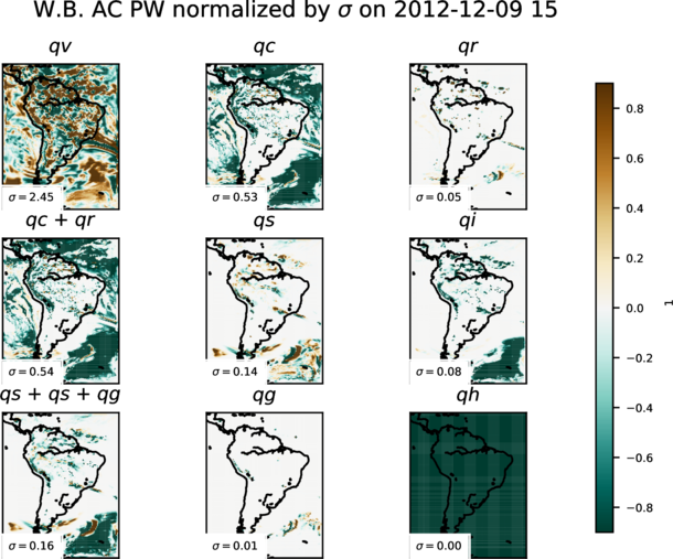
Water vapor balance terms
These covers the different column integrated terms of the water balance equation. The equation of the water vapour budget:

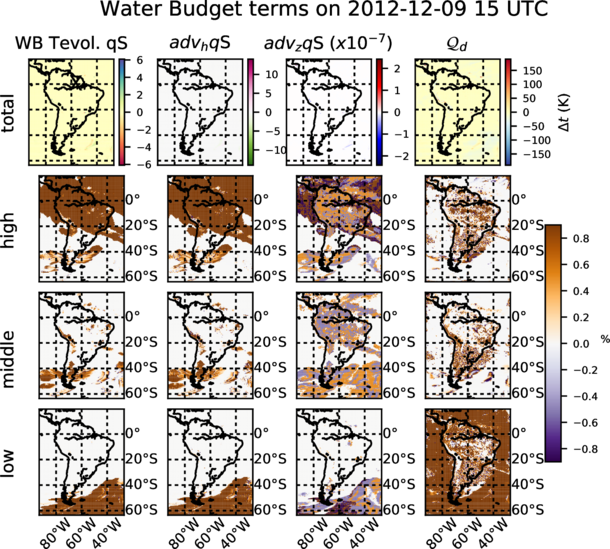
Where q stands for either of the five water species concentration (vapor, snow, ice, rain and liquid), Vh stands for horizontal wind speed, w stands for the vertical wind speed and MP for the loss or gain of water due to cloud microphysical processes. The term in the left-hand side of the equation represents the water species tendency (TEN or PW), referring to the difference between q at the model previous time step and at the end of the actual time step, divided by the time step. TEN equals to the horizontal advection (HOR or 'F', first term in right-hand side of the equation), the vertical advection (VER or 'Z', second term in right-hand side) and the sources (SO) or sink (SI) of atmospheric water due to microphysical processes (MP). All terms are expressed in kgkg-1s-1. However, SO, and SI ca not be provided because they are micro-physics dependent an make difficult to provide a general formula for them.
In order to obtain the total column mass of water due to each term (in units of mm), it is applied to each term of eq. 26 (similarly as in 5):
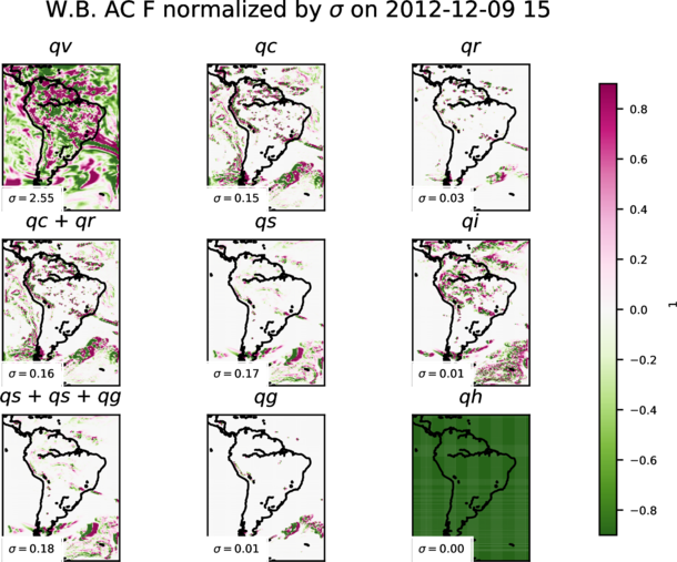
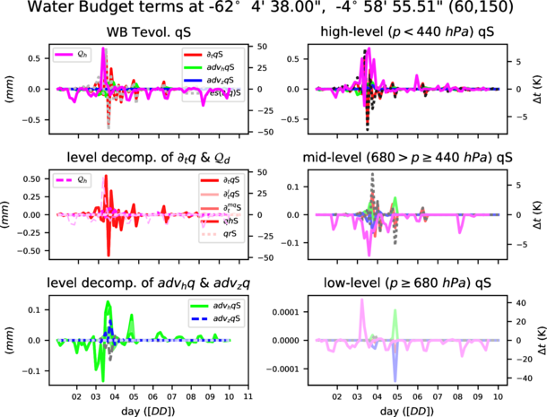
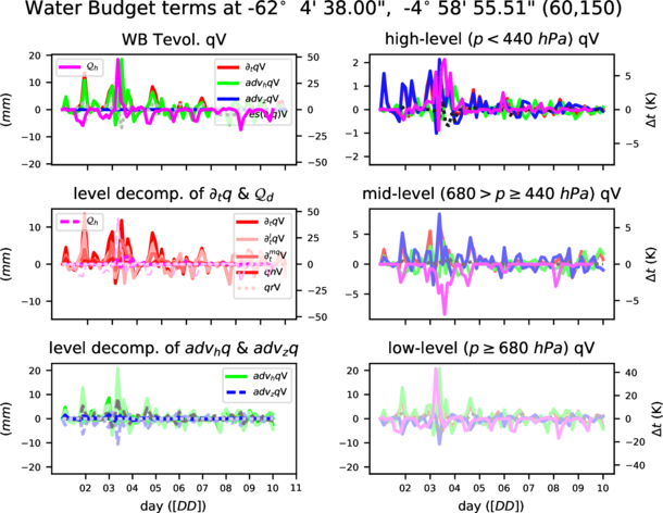
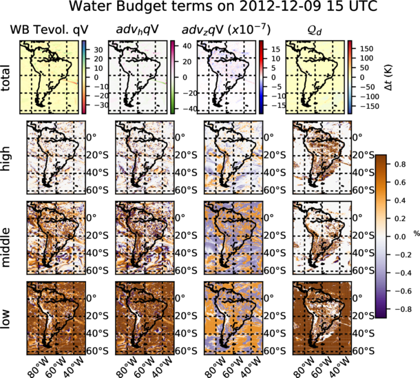
Following the methodology of Huang et al. (2014) and Yang et al. (2011), Fita and Flaounas (2018) implemented the water budget terms in a new module in WRF in order to allow the computation of the terms during model integration. For the CORDEX module, only the vertically integrated variables will be implemented. Microphysics processes depends on the micro-physics scheme used during model run. It is know the the budget is closed, thus, residual of the terms must be the micor-phsyics term. Due to the complexity of each micro-physics scheme and the impossibility to generalize the calculation, the accumulation of diabatic heating from the micro-physics scheme is provided as a proxy. All water species decomposition is shown in figures 7 and 8 It has also been grouped by vertical levels as it is done with the clouds: p ≥ 68000 P a, 40000 ≤ p < 68000 P a, p < 40000 P a. Decomposition of each term is shown for water vapour qv and snow in figures from 9 to 12.
tfog: time of presence of fog
A diagnostic of visibility has been introduced. From it, one can define fog as that moment where the visibility is lower than 1 km (WMO, 2010).
tfog accounts for the time in which the grid point has visibility lower than 1 km (see equation 27)
where Nfog: number of time steps where visibility was below 1 km. δt: model time step (s)
fogvisblty: visibility inside fog
A diagnostic of visibility is introduced in order to provide a diagnostic for fog. Three different methods have been introduced:
- K84: Visibility is computed by means of liquid water (
QCLOUD) and ice (QICE) concentrations. Following (Bergot et al., 2007) fog appears when there are liquid and/or ice water species at the lowest level. Visibility using (see equation 28, Kunkel 1984) formula is computed on that grid points where fog appeared. Method selected withvisibility_diag = 1
where qc: liquid water (cloud) mixing ratio (kgkg-1), qi: ice mixing ratio (kgkg-1). Visibility values are in km
- RUC: Visibility is computed using relative humidity (hur) as it is implemented in the RUC model (see equation 29, Smirnova et al. 2000). Method selected with
visibility_diag = 2
where rh: relative humidity (1) and can be from surface or first model layer. Visibility values are in km
- FRAM-L: Visibility is computed using relative humidity (hur) after (see equation 30, Gultepe and Milbrandt, 2010). In this work, it is proposed a probabilistic approach to the computation of the visibility in three different bins: 95% , 50% and 5% of probability to get certain visibility (for rh > 30%). As a matter of compromise, the calculation for the 50% of probability has been chosen as the preferred one. Thus, this method provides the visibility that might be with a 50% of probability. Method selected with
visibility_diag = 3(default)
where rh: relative humidity (1) and can be from surface or first model layer. Visibility values are in km
Provided values in the output are the minimum, maximum and mean values within output time-steps
Different choices are controlled throughout namelist.input variables: visibility_diag method of visibility computation, fogvars source of the relative humidity. From first model layer (hur) fogvars=1 (default), surface (hurs) fogvars=2. See some preliminary results in figure 13
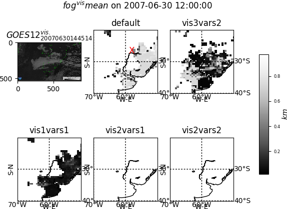
It is known that certain methods of visibility relay on numerical adjustments on certain observational data taken under certain circumstances and places (e.g.: for FRAM-L adjusted values come from observations from a Canadian airport). It would be desirable to provide a more generic all places/purposes (if possible) approach. Take this value with certain care
Missing variables
There are certain variables from CORDEX ‘Tier1’ which could not yet be introduced
wsgsmax100: Daily Maximum Near-Surface Wind Speed of Gust at 100 m
The wind gust at 100 m is understood that should follow similar processes that the wind gust at the surface (like in wsgsmax). At this version of the module there has not been considered to be included in the search for the right equations and approximations.
ic_lightning, cg_lightning, tot_lightning: intra-cloud, ground and total lightning flashes
There is lightning scheme implementation in WRF. (lightning_option among other from namelist.input). It might require some adjustment prior it’s use. It does not sees to provide a wolrdwide cloud/ground discrimination
Optimization
Regional climate dynamical downscaling experiments require long continuous simulations. Thus, model performance in terms of speed of integration are crucial. First version of the module (v1.0) was known to introduce a lose in time-step speed of integration of about 40\% slower (highly dependent on HPC, model configuration and domain). In order to improve model performance when the module is activated, an enhanced version of the module (v1.1) was prepared. In this new version, a series of pre-compilation flags were activated, with which, user can choose the level of complexity and amount of variables to obtain. Doing it in this way instead via regular namelist options, two main goals are obtained: (1) reduce the amount of variables to be kept in memory during model execution and (2) reduce the amount of conditions (mainly avoiding IF statements) to be check at each execution step.
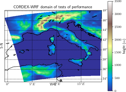
A domain (see figure 15 and table for details) has been set-up to perform short runs (5 days) to check the optimization of the WRF module with the pre-compilation flags for the compilation of the model. Simulations are run in a single node (to avoid non-homogeneous communications among nodes of the cluster) and with the model compiled (intel compiler v16.0.4.258) only in distributed memory mode on CRAY XE6/XC40 machine under SUSE Linux Enterprise Server 12 (x86_64) version 12 patchlevel = 3.
| Domain characteristic | value |
|---|---|
| projection | lat-lon |
| central point | N 48.0522°, 23.07623° E |
| refx,y | 118, 99 |
| polelat,lon | N 39.25000°, 18.00000° E |
| standard longitude | 18.00000° W |
| grid-points | 100x100 |
| resolution | 0.13750x0.13750° |
| vertical levels | 50 |
| time-step | 15 s |
Time measurements are done with the elapsed time-step of each model integration obtained from the standard output of the model run (rsl.error.0000 WRF ASCII file, see in figure 16). In this file, WRF users can get the elapsed time for all the time-steps of the model. Different peaks of slower time-steps are seen with coincidence to Input/Output file operations and when different physical schemes (mainly the radiative scheme) are activated on a given frequency. With 5-days simulations and time-steps of 50 seconds, one obtain more than 10,0000 time-steps. Thus, the mean time step is computed as the average of all the 23,221 time-steps of the simulation.
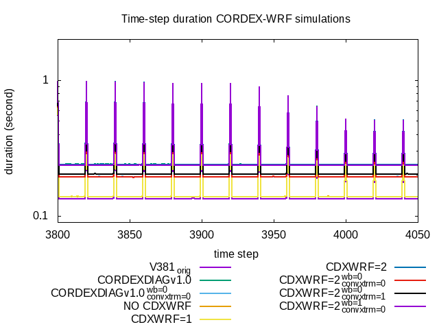
In order to know sensitivity of the model performance to the different configurations and options of the module, a series of simulations are performed (see table below). The first simulation (labeled v381orig) and used as reference, is the simulation with the original version of the model (here version 3.8.1) without the module. The first version of the module (v1.0, labelled v10) with all the extra calculations (water budget components, namelist option wb_diag=1 and extremes of convective parameters, namelist option convxtrm_diag=1). A simulation with version 1.0 but without extra computations (v10_NOwbconvxtrn). Another with the new version (v1.1) without the setting of pre-compilation parameter CDXWRF (labelled v11_NOCDXWRF). Another with version 1.1 with pre-compilation parameter CXWRF=1 (v11_CDXWRF1). Another with pre-compilation parameter CDXWRF=2 and computing all extra calculations (v11_CDXWRF2). Finally three additional more without any extra calculation (v11_CDXWRF2_00), without calculation of extra water-budget terms (v11_CDXWRF2_01) and only without extremes from convection indices (V11_CDXWRF2_10).
| label | module version | description | mean time (second) | % increment |
|---|---|---|---|---|
| v381orig | - | original WRF 3.8.1 version of the code | 0.163376306424 | 1 |
| v10 | 1.0 | wb_diag=1 & convxtrm_diag=1
|
0.26841433724 | 64.3 |
| v10_NOwbconvxtrm | 1.0 | wb_diag=0 & convxtrm_diag=0
|
0.223246675347 | 36.6 |
| v11_NOCDXWRF | 1.1 | without CDXWRF
|
0.167709105469 | 2.7 |
| v11_CDXWRF1 | 1.1 | CDXWRF=1
|
0.167785992187 | 2.7 |
| v11_CDXWRF2 | 1.1 | CDXWRF=2
|
0.267609857639 | 63.8 |
| v11_CDXWRF2_00 | 1.1 | CDXWRF=2 wb_diag=0 & convxtrm_diag=0
|
0.22327053342 | 36.7 |
| v11_CDXWRF2_01 | 1.1 | CDXWRF=2 wb_diag=0 & convxtrm_diag=1
|
0.233002554688 | 42.6 |
| v11_CDXWRF2_10 | 1.1 | CDXWRF=2 wb_diag=1 & convxtrm_diag=0
|
0.26442043099 | 61.8 |
Results show that all the simulations where the module has been added are slower than the simulation with the original version of the code (v381orig, <t>= 0.1634 s). Simulation with version 1.1 of the module without pre-compilation flag CDXWRF (v11_NOCDXWRF, <t>= 0.1677 s) is the second more fast begin faster than the similar configuration with the original version of the module without the extra calculation (v10_NOwbconvxtrm, <t>= 0.2232 s). In both versions the simulation is similarly slow when all the extra calculations are performed (v10 <t>= 0.26841433724 s, v11_CDXWRF2 <t>= 0.2676 s). The heaviest part of the module is related to the water budget computation since with respect the simulation without extra calculations (v11_CDXWRF2_00, <t>= 0.2233 s) there is an increase of only about 4% of mean time step when only statistics of extreme convective indices is activated (v11_CDXWRF2_01, <t>= 0.2330 s) with respect an increase of 18% when only water-budget terms are included (v11_CDXWRF2_10, <t>= 0.2644 s).
These results show the important effect on model performance of the number of variables included during the integration (included in the derived type grid) which will reduce the required amount of memory.
Accordingly to the value given to the pre-compilation variable CDXWRF one obtains:
- Without adding the variable: all CORDEX 'Core' variables
-
CDXWRF=1CORDEX 'Tier' variables: clgvi, clhvi, zmla, [cape/cin/zlfc/plfc/lidx]{min/max/mean} -
CDXWRF=2The same as with CDXWRF=1 and additional variables: ua, va, ws, ta, press, zg, hur, hus, tfog, fogvisblty{min/max/mean}, tds{min/max/mean} and the Water-Budget relarted ones: wbacdiabh, wbacpw, wbacpw[c/r/s/i/g/h], wbacf, wbacf[c/r/s/i/g/h], wbacz, wbacz[c/r/s/i/g/h], wbacdiabh{l/m/h}, wbacpw{l/m/h}, wbacpw{l/m/h}[c/r/s/i/g/h], wbacf{l/m/h}, wbacf{l/m/h}[c/r/s/i/g/h], wbacz{l/m/h}, wbacz{l/m/h}[c/r/s/i/g/h]
Simultanesouly, one needs to modify the Registry/registry.cordex accordingly to the value of CDXWRF:
- Without adding CDXWRF, nothing needs to be changed
- Adding
CDXWRF=1, one needs to remove the comment##CDXWRF1##at the beginning of the line of the definition of certain variables - Adding
CDXWRF=2, one needs to remove the comment##CDXWRF1##and##CDXWRF2##at the beginning of the line of the definition of certain variables
Additionally, now interpolation of 3D fields to pressure levels is only done at the same frequency as the output of the wrfpress file.
Others
It will be some other hard work to do related to it.
New variables
Pretty sure that as we get closer to stake-holders, decision makers, impact and mitigation communities more variables will arise... keep in touch !?
CF-compilant file
WRF does not provide a real CF-compilant file format. It would be necessary to add at least at the output (at least on the wrfcdx_d<domain>_<date> file):
- time variable: CF-version of variable with times in the file
- atrtributes: WRF does not provide variables with standard attributes like: standar_name, long_name, ...
Instantaneous valuess
As an additional work, all the instantaneous variables used for the different accumuluations and extremes, can also be retrieved. It is only necessary to:
- Give an output unit on the
registry.cordex(see instructions at the end of the file) - Uncomment in the code (
phys/module_diagnostics_dirver.Fandmodule_diag_cordex.F), the commented lines with the key word:INSTVALS - re-compile WRF after cleaning all the code (due to the modification in the
Registry)
WRF output names
Open page for the list of variables added with the module CDXWRFout
Acknowledgements
All the coders of WRF, LMDZ, ORCHIDEE are acknowledged for their work on the developing and maintaining of the models. M. A. Jiménez from Universitat de les Illes Balears (UIB) is acknowledged by her explanations on certain PBL calculations. J. Milovac from U. Hohenheim for her comments is also acknowledged. D. Argüeso from UIB. E. Katragkou and G. Sofiadis from U. Thesaloniki, T. Μ. Giannaros from National Observatory of Athens, T. Lorenz from Uni Research, the Bjerknes Centre and J. Milovac from U. Hohenheim for their assistance in the additional tests. V. Galligani, J. Ruiz and M. Sebastián from CIMA. All the development of the module has been carried out in the CIMA `hydra' cluster, L. Fita thanks the IT support for their work.
References
- Bergot, T., Terradellas, E., Cuxart, J., Mira, A., Liechti, O., Mueller, M., and Nielsen, N. W. (2007). Intercomparison of single-column numerical models for the prediction of radiation fog. Journal of Applied Meteorology and Climatology, 46(4):504–521.
- Brasseur, O. (2001). Development and application of a physical approach to estimating wind gusts. Monthly Weather Review, 129(1):5–25.
- Fita, L., Fernández, J., and García-Díez, M. (2010). Clwrf: Wrf modifications for regional climate simulation under future scenarios. Proceedings of 11th WRF Users’ Workshop.
- Fita, L. and Flaounas, E. (2018). Medicanes as subtropical cyclones: the december 2005 case from the perspective of surface pressure tendency diagnostics and atmospheric water budget. Q. J. Royal Met. Soc., doi: 10.1002/qj.3273
- García-Díez, M., Fernández, J., Fita, L., and Yagüe, C. (2013). Seasonal dependence of wrf model biases and sensitivity to pbl schemes over europe. Q. J. of Roy. Met. Soc., 139:501–514.
- Garratt, J. (1992). The Atmospheric Boundary Layer. Cambridge Univ. Press, Cambridge, U.K.
- Hourdin, F., Musat, I., Bony, S., Braconnot, P., Codron, F., Dufresne, J.-L., Fairhead, L., Filiberti, M.-A., Friedlingstein, P., Grandpeix, J.-Y., Krinner, G., LeVan, P., Li, Z.-X., and Lott, F. (2006). The LMDZ4 general circulation model: climate performance and sensitivity to parametrized physics with emphasis on tropical convection. Clim. Dyn., 27(7-8):787–813.
- Huang, H.-L., Yang, M.-J., and Sui, C.-H. (2014). Water budget and precipitation efficiency of typhoon Morakot (2009). J. Atmos. Sci., 71:112–129.
- Jourdier, B. (2015). Ressource éolienne en france métropolitaine : méthodes dâĂŹévaluation du potentiel, variabilité et tendances. Climatologie: École Doctorale Polytechnique, 2015. Français. ph:+33 01238226, pages 1–229.
- Kunkel, B. A. (1984). Parameterization of droplet terminal velocity and extinction coefficient in fog models. Journal of Climate and Applied Meteorology, 23(1):34–41.
- Monteith, J. L. (1965). Evaporation and environment. the state and movement of water in living organisms. 19th Symp. Soc. Exp. Biol, pages 205–234.
- Nielsen-Gammon, J. W., Powell, C. L., Mahoney, M. J., Angevine, W. M., Senff, C., White, A., Berkowitz, C., Doran, C., and Knupp, K. (2008). Multisensor estimation of mixing heights over a coastal city. Journal of Applied Meteorology and Climatology, 47(1):27–43.
- Skamarock, W. C., Klemp, J. B., Dudhia, J., Gill, D. O., Duda, D. M. B. M. G., Huang, X.-Y., Wang, W., and Powers, J. G. (2008). A description of the advanced research wrf version 3. NCAR TECHNICAL NOTE, 475:NCAR/TNÂŋ475+STR.
- Smirnova, T. G., Benjamin, S. G., and Brown, J. M. (2000). Case study verification of ruc/maps fog and visibility forecasts. Preprints, 9 th Conference on Aviation, Range, and Aerospace Meteorlogy, AMS, Orlando, FL, Sep. 2000, 2.3:6.
- WMO (2010). Guide to meteorological instruments and methods of observation. Weather - Climate - Weather, pages
1–176.
- Yang, M. J., Braun, S. A., and Chen, D.-S. (2011). Water budget of typhoon nari (2001). Mon. Wather Rev., 139:3809–3828.


