CDXWRFcore

Core variables

UNDER CONSTRUCTION

These are the basic variables required by CORDEX. Most of them are standard fields and therefore tend to require simple calculations from the currently available variables from the WRF model. These variables are obtained by setting the pre-compilation flag CORDEXDIAG, and will appear in two different files: 3D variables at pressure levels (the WRF model internally interpolate them since it uses the η coordinate in the vertical) will appear in the output file with the 23rd stream (mainly called wrfpress), and the 2D variables in the module's output file wrfcdx.

3D at pressure-levels

These are the additional variables which have been added into the WRF pressure-level integration module. Their values will be written in the 23rd output stream in addition to the ones currently available. All of them are instantaneous values (See in table 1 a description of the variables in pressure levels added).

Table 1: Description of CORDEX additional pressure interpolated variables provided with the module

CF name	WRF name	description	units
hus	HUS_PL	specific humidity	1
wa	W_PL	vertical wind speed	ms-1
ua	UER_PL	Earth-rotated wind x-component	ms-1
va	VER_PL	Earth-rotated wind y-component	ms-1
ws	WS_PL	wind speed	ms-1

hus: humidity

3D atmospheric specific humidity (hus) 1 and relative humidity (hur) are computed at the unstaggered model η levels. Specific humidity is simply obtained from water vapor mixing ratio using equation 2 (named QV AP OR in WRF). Relative humidity can be obtained following the Clausius-Clapeyron formula and its approximation from the well-known August-Roche-Magnus formula for saturated water vapor pressure.

where r_v: mixing ratio (kgkg^-1), with tempC: being temperature in degree Celsius (^◦C), presshPa: pressure (hPa), es: saturated water vapor pressure (hPa), ws: saturated mixing ratio (kgkg-1).

press: air-pressure

WRF model integrates the perturbation of the pressure field from a reference one. Thus to obtain the full pressure at unstaggered model η levels, it is required to combine two different fields as shown in equation 5,

where PB, WRF base pressure (Pa), P, WRF perturbation pressure (Pa)

ta: air-temperature

This variable states for the 3D atmospheric temperature on unstaggered model η levels. WRF model equations are based on the perturbation of potential temperature, therefore a conversion to actual temperature is required, and it is performed as indicated by equation 6,

where T, WRF temperature (K, which is as potential temperature), PB, WRF base pressure (Pa), P, WRF perturbation pressure (Pa), p0: pressure reference 100000 (Pa)

ua/va: Earth roteted wind components

These variables state for the 3D atmospheric wind components following Earth coordinates on standard model η levels. WRF model equations use the Arakawa-C horizonatally staggered grid with wind components following the grid direction. In order to get actual winds following the Earth geographical coordinates, a transformation shown in equation 7 is required,

where U_stg: x-staggered WRF eastward wind (ms^-1, [1,dimx+1]), V_stg: y-staggered WRF northward wind (ms ^-1, [1,dimy+1]), U_unstg: unstaggered WRF eastward wind (m^s-1, [1,dimx]), V^unstg: unstaggered WRF northward wind (ms^-1, [1,dimy]), cosa: local cosine of map rotation (1), sina: local sine of map rotation (1).

zg: geopotential height

As in the case of air-pressure, WRF model also integrates the perturbation of the geopotential field from a reference or base one. Thus to obtain the full geopotential height on staggered model η levels, it is required to combine the two WRF fields andit is also destaggered as it is shown in equation 8,

where PHB, WRF base geopotential height (m²s^-2), PH, WRF perturbation geopotential height (m²s^-2), zg_staggered: staggered geopotential height k=[1, dimz+1], zg: un-staggered geopotential height k=[1, dimz]

2-dimensional

Here is provided the list of the the added 2-dimensional CORDEX variables. Some of them are diagnosed as a combination of 3-dimensional variables, some are required as instantaneous values, and others as statistics. The fact that the module provides 2D variables online using 3D fields, shows one more key advantage of the module related to disk space. Thanks to these online calculations when using the module, a user does not need anymore to store large amount of 3D data from the model in order to post-process them. This reduces the requirements of disk space by a factor of around 2.

pr, prc, prl, prsh, prsn: precipitation fluxes

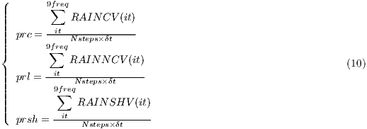
The total precipitation flux (pr) is computed as the sum of all types of precipitation fields in the model accumulated along the 9th stream output frequency (9freq) divided by this period of time (9freq), as it is shown in equation 9,

where RAINCV: instantaneous precipitation from cumulus scheme (kgm^-2), RAINNCV: instantaneous precipitation from microphysics scheme (kgm^-2), RAINSHV: instantaneous precipitation from shallow-cumulus scheme (kgm^-2), Nsteps: number of time steps, and δt: time step length (s) to achieve the 9th stream frequency output time (9f req = N steps × δt). In this version, the computation of the accumulated values does not take into account configurations of the model with adaptive time-step. When adaptive time-step is used, we strongly discourage the use of these variables.

Each individual precipitation flux is also provided as:

Solid precipitation flux (prsn) only accounts for frozen precipitation. Depending on the selected micro-physics scheme chosen in the `namelist', this variable might account for the precipitation of snow, graupel and hail. It is computed as it is shown in equation 11,

where prins: instantaneous total precipitation (kg^-2, previously obtained), SR: fraction of solid precipitation (%, variable provided by WRF).

Radiative flux

Surface upwelling shortwave radiation flux (rsus, W gm −2 ) and surface upwelling longwave radiation flux (rlus, W gm^-2) are understood as the shortwave and longwave radiation from Earth's surface. They are directly provided by radiation schemes CAM (Community Atmosphere Model) and RRTMG (Rapid Radiative Transfer Model) (sw_ra_scheme = 3,4) as instantaneous variables swupb and slupb. When there is no use of such schemes, it is recommended to use the `generic' definition instead (rsusgen, rlusgen, see in next section). Statistical retrieval for the surface fluxes follows the same methodology as for the precipitation fluxes.

Outgoing radiative fluxes at top the atmosphere are also provided being `rsut' for mean Top of the Atmosphere (TOA) outgoing shortwave radiation (in Wgm<sup>-2</sup>) and `rlut' for longwave. However there is not a `generic' implementation of these variables.

sund: duration of sunshine

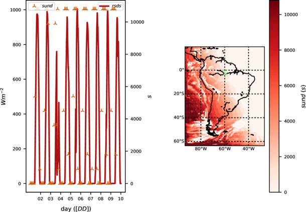
This variable accounts for the the sum of the time for which the direct solar irradiance (downwelling short-wave radiation, rsds) exceeds 120 Wm^-2 (WMO, 2010a) implemented following equation 12 and provided in seconds. In order to provide an example of the correct implementation of this diagnostics preliminary results are shown in figure 2. The figure shows the `sund' values and compare them with the incoming solar radiation. It is shown how the `sund' values vary accordingly to the moment of the day with zero values during night (left panel) or persistent totally cloud covered regions (map at the right panel)

where SWDOWN: downward shortwave radiation (W m^-2), δt: time-step length (s).

Figure 2: Temporal evolution at S 62^◦ 4' 38.00", 4^◦ 58' 55.51" W (left panel) of shortwave downward radiation (rsds, red line, left y-axis) and sunshine duration for a 3-hourly 9freq (sund, stars, right y-axis). Sunshine length map on 2012-12-09 at 15 UTC. X denotes position of the temporal evolution

tauuv: surface downward wind stress

Instantaneous surface downward wind stress at 10m accounts for the force that winds exerts on the Earth's surface. It is implemented following the equation 13

where, CD: drag coefficient (1), uas: Earth-rotated eastward 10 m surface wind (ms^-1), vas: Earth-rotated northward 10 m surface wind (ms^-1). The drag coefficient is non-zero only for certain options of the surface layer physics (sf_sfclay_physics parameter in the namelist): 1 (MM5-similarity), or 5 (MYNN surface layer). A `generic' formulation has been introduced when these schemes are not used.

psl: sea level pressure

This variable accounts for the instantaneous pressure extrapolated to the sea level. It represents the value of the pressure without the presence of orography. In order to provide a framework ready to implement different methodologies, three different methods have already been implemented. The choice of the method can be controlled by a new namelist.input parameter labeled psl_diag in cordex section. The implemented methods are:

• The hydrostatic-Shuell method (Stackpole and Cooley, 1970) already implemented in the the module phys/module_diag_afwa.F, assuming a constant lapse-rate of -6.5 Kkm^-1 , selected when in WRF 'cordex' namelist section setting the parameter [psl_diag = 1]
• The 'ptarget' method (Benjamin and Miller, 1990) that uses smoothed surface pressure and a target upper-level pressure, already implemented in the WRF post-processing tool called p_interp.F90 [psl_diag = 2]
• The ECMWF method (Yesad, 2015) taken from the Laboratoire de Météorologie Dynamique GCM (LMDZ; Hourdin et al., 2006) from the module pppmer.F90, following the methodology by Mats Hamrud and Philippe Courtier from ECMWF [psl_diag = 3]

According to the CORDEX specifications, the default method is the ECMWF method. When choosing the `ptarget' method (psl_diag = 2), also the degree of smoothing of the surface using the surrounding nine point average can be chosen by selecting a number of smoothing passes (psmooth, default 5), and the upper pressure that has to be used as the target (ptarget, default 700 hP a).

Figure 3: Sea level pressure estimates following the hydrostatic-Shuell method at a given time step (psl^shuell, upper left), ptarget (psl^ptarget, upper middle) and ECMWF (psl^ecmwf, upper right). Bottom panels show differences between methods psl^shuell - psl^ptarget (bottom left), psl^shuell - psl^ecmwf (bottom middle) and psl^ptarget - psl^ecmwf (bottom right)

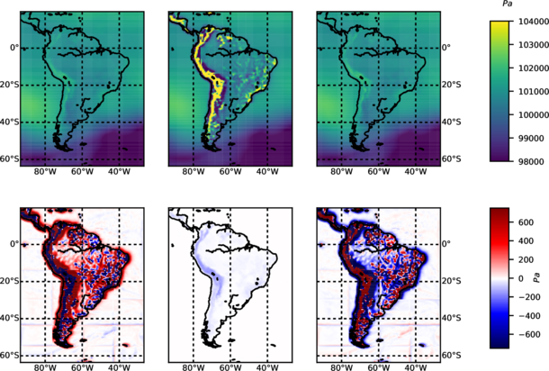
Figure 3 shows the different outcomes applying each method. There are some problems with the p-target method in both psl estimates (mountain ranges can still be inferred) and borders for each parallel process (lines in figures showing differences among methods) when the spatial smoothing is applied. Lines showing the limits of the parallel processes appear because one can not obtain the proper values from outside the correspondent tile of the domain associated with each individual parallel process.

Cloud derived variables

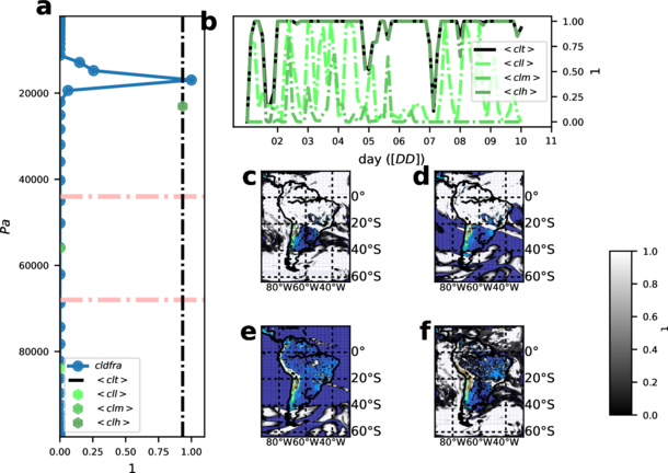
Four cloud derived variables are required by CORDEX: the total cloudiness (clt) and the cloudiness for each grid point at three different vertical layers above ground (low: p ≥ 680h Pa, labeled cll; medium: 680 < p ≥ 400 hPa, clm; high: p < 400 hPa, clh). These cloud diagnostics are provided as mean values.

The module computes these variables taking the cloud fraction of a given grid cell and level as input. The cloud fraction in WRF is computed by the radiative scheme, and it is called at a frequency given by radt parameter in WRF namelist.

Due to the large computational cost of the radiative scheme, radt usually is larger than the time-step of the simulation. This determines when cloud fraction is also actualized to meet the evolved atmospheric conditions. Cloud fractions can be computed in the model using different methodologies. It would be possible to make available these methodologies as another choice in the namelist section and then compute the cloud fraction at each time-step. However, in order to be consistent with the radiative cloud effects that the simulation is experiencing, this method was discarded. Thus, the cloud values provided by the module follow the same frequency of refreshing rate as the one set for radiation in the namelist level (radt value). The most common implementation of `clt' found in other models (in particular most GCMs) assumes `random overlapping'. Random overlapping assumes that adjacent cloud layers are from the same system, hence are maximumly overlapped (Geleyn and Hollingsworth, 1979). In the module, the methodology from the GCM LMDZ was implemented. In this GCM, calculation of the total cloudiness and different layers' cloudiness is done inside the subroutine newmicro.f90. The method basically consists in a product of the consecutive non-zero values of cloud fraction as it is shown in equation 14,

where CLDFRAC: cloud fraction (1) at each vertical level, zclear: clear-sky value (1), zcloud: cloud-sky value (1), ZEPSEC: value for very tiny number. Same methodology as in equation 14 is applied for the diagnostic of `clh', `clm' and `cll' but splitting by corresponding pressure layers. The figure 4 illustrates the result of the implementation and compare the results with the actual values of the cloud fraction (a and b panels) as well as the different cloud distribution (panels c to f).

Figure 4: Vertical distribution of cloud fraction and the different cloud layers on 2012-12-09 at 15 UTC at S 62^◦ 4' 38.00", 4^◦ 58' 55.51" W (a): cloud fraction (cldf ra, full circles with line in blue), mean total cloud fraction (clt, vertical dashed line), mean low-level cloud fraction (cll p ≥ 680 hP a, dark green hexagon), mean mid-level (clm 680 < p ≥ 440 hP a, green hexagon), mean high-level (clh p < 440 hP a, clear green hexagon). Temporal evolution of cloud layers at the given point (b). Map of clt with colored topography beneath to show-up cloud extent (c), map of clh (d), map of clm (e) and map of cll (f)

Wind derived variables

CORDEX requires two wind-derived diagnostics: the daily maximum near-surface wind speed of gust (wsgsmax) and the daily maximum wind speed of gust at 100m above ground (wsgsmax100). These variables can not be retrieved by post-processing the standard output since they require the combination of different variables (some of them not available from the model output) and have to be produced as a maximum value. The module provides different ways to compute them under certain limitations.

wsgsmax: maximum near-surface wind speed of gust

The wind gust accounts for the wind from upper levels that is projected to the surface due to instability within the planetary boundary layer. In the current version of the module two complementary methods of diagnosing the variable have been implemented (resultant winds are Earth-rotated). The choice between the two methods is done by the parameter labeled wsgs_diag (in cordex section), with the default value set to 1. The implemented methods are:

• The Brasseur method [wsgs_diag = 1]: An implementation of wind gust considering Turbulent Kinetic Energy (TKE) estimates and stability defined by virtual temperature (θ v ) as indicated in equation 15 following Brasseur (2001). Implementation is adapted from a version already introduced in the CLimate WRF ([clWRF]; Fita et al., 2010),

where TKE: Turbulent Kinetic Energy (m2s^-2), θ_v: virtual potential temperature (K). z_p height of the considered parcel (m, maximum height which satisfies equation 15), ∆θ_v (z): variation of θ>SUB>v</SUB> over a given layer (Km^-1).

• The AFWA method [wsgs_diag = 2]: An implementation adopted from the WRF module module_diag_afwa.F which calculates the wind gust that only occurs as a blending of upper-level winds zagl (around 1 km above ground; zagl(k₁₀₀₀) ≥ 1000 m, see equation 16) when precipitation intensity per hour is above a given maximum value, prate mm

where va: air wind (ms^-1), zagl: height above ground (m), k_₁₀₀₀: vertical level at which zagl is equal or above 1000 m. prate mm), va blend : blended wind (ms^-1) hr: hourly precipitation rate (mmh^-1)

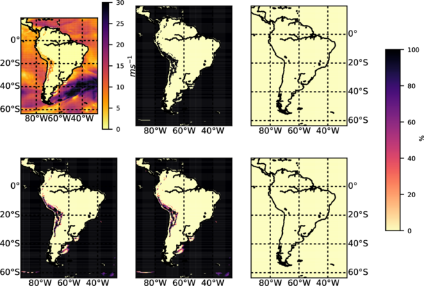
The two methods provide wind gust estimation (WGE) from two different perspectives: mechanic and convective. In order to take into account both perspectives, additional variables: totwsgsmax (total maximum wind-gust speed at surface), totugsmax (total maximum wind-gust eastward speed at surface), totvgsmax (total maximum wind-gust northward speed at surface), and totwsgspercen (percentage of time steps along 9freq in which grid point got wind gust (%). Figure 5 shows the outcomes when applying each method. It is shown how wind gust is mainly originated by instability, with a minor impact of heavy precipitation events at the given time. Furthermore, in the bottom panel it is shown how wind-gusts are highly frequent above the sea in comparison to the low frequency above continental flat areas (Andes mountain range exhibits high occurrence of wind gust).

Figure 5: Near surface wind gust estimates on 2012 December the 9th at 15 UTC. 3h-maximum total wind gust strength (wsgsmax^tot, top left), percentage of wsgsmax^tot following the Brasseur method (wsgsmax^b01, top middle), percentage following the AFWA-heavy precipitation implementation (wsgsmax^hp, top right), percentage of time steps where grid point got total wind gust (bottom left), percentage of time steps where grid point got wsgsmax^b01 (bottom middle), percentage due to wsgsmax^hp (bottom right)

wsgsmax100: daily maximum wind speed of gust at 100 m

The calculation of wind gust at 100 m should follow a similar implementation used for calculating the wsgsmax, but at 100 m. An extrapolation of such turbulent phenomena would require a complete new set of equations which have not been placed yet. However, it could be considered as first approach to take the same wind gust as the one at the surface (when it is deflected from above 100 m). The assumption would be that the wind gust at 100 m would correspond to the deflected wind on its `way' to the surface. Instead, as a way to complement, the estimation of maximum wind speed at 100 m is provided. Provided wind components are also Earth-rotated. Three different methods have been implemented. Two following per-assumed vertical wind profiles (after PhD thesis Jourdier, 2015) and a third one following Monin-Obukhov theory to estimate the wind components above ground. These three methods are chosen by the namelist parameter labeled wsz100_diag. Its default value is 1. The implemented methods are:

• [wsz100_diag = 1], following the power-law wind vertical distribution as depicted in equation 17 using the upper-<>level atmospheric wind speed below (k^<₁₀₀) and above (k^>₁₀₀) the height above ground of 100 m (zagl), va 100

• [wsz100_diag = 2], following logarithmic-law wind vertical distribution, as it is depicted in equation 18, using > upper-level atmospheric wind speed below (k^<₁₀₀) and above (k^<₁₀₀) the height above ground of 100 m (zagl)

• [wsz100_diag = 3], following Monin-Obukhov theory. User should keep in mind that this method is not useful for heights larger than few decimeters (z > 80 m). The wind at given height is extrapolated following turbulent mechanisms. As it is shown in equation 19, surface wind speed is used as surrogate to estimate 100 m wind direction (θ₁₀ = tan⁻¹(uas, vas), without considering Eckman pumping, or other effects on wind direction). In this implementation u ∗ in similarity theory is taken as WRF estimates UST, Monin-Obukhov length (LO) as the WRF values RMOL, roughness length (z₀) as WRF thermal time-varying roughness length ZNT,

where Ψ_M: stability function after (Businger et al., 1971), UST: u^∗ in similarity theory (ms^-1), z₀: roughness length (m), U10, V10: 10-m wind speed (ms^-1 ), theta₁₀: 10-m wind speed direction (rad), ua₁₀₀: 100 m eastward wind speed (ms^-1), va₁₀₀: 100 m northward wind speed (ms^-1). Note the absence of correction in wind direction to Ekman pumping or other turbulence effects.

The user can also select the height at which the estimation is computed throughout the namelist parameter z100m_wind [100 m as default value].

Figure 6 shows different preliminary results using the three different approximations. It is illustrated (a panel) how wind-gusts are larger than the 10-m diagnostic winds, and also the difference is larger when using Monin-Obukhov how method compared to the two others methods. Certain problems (too small Monin-Obukhov length) are recognized when applying Monin-Obukhov for extrapolating wind at 100 m, which is shown in panel b, where wind gusts appear to be strong as 80 ms^-1. Therefore a user is advised to use this method with care.

[[Archivo:test_wsz100.png|frame|50px|Figure 6: 100 m wind estimates. Comparison between upper-level winds and estimation on 2012-12-09 at 15 UTC at S 62^◦ 4' 38.00", 4^◦ 58' 55.51" W (a): 3h-maximum eastward wind (red) at 100 m by power-law (uzmax^pl, star marker), Monin-Obukhov theory (uzmax^mo, cross) by logarithmic law (uzmax^ll, sum) 10-m wind value (uas, filled triangle) and upper-level winds (ua, filled circles with line), also for the northward component (green). Temporal evolution of wind speed (b) with all approximations and upper-level winds at the closest vertical level at 100 m (on log-y scale, <z>= 107.1 m on average). Maps of three estimations: power-law (c), Monin-Obukhov (d), logarithmic-law (e) with the blue cross showing the point of previous figures. Vertical distribution of winds at the given point in Wind rose-like representation (f)

Vertically integrated variables

The instantaneous vertically integrated amount of water vapor (prw), liquid condensed water species (clwvi), ice species (clivi), graupel (clgvi), hail (clhvi) are the vertically integrated amounts of each species along the vertical column (density weighted) over each grid point. They are provided using the same implementation as those in p_interp.F - WRF tool for vertical interpolation. The general equation following WRF standard variables is:

where clvivar: the column vertically integrated variable's CF-compliant name (prw, clwvi, clivi, clgvi, or clhvi), MU: perturbation dry air mass in column (Pa), MUB: base-state dry air mass in column (Pa), g: gravity (ms^-2), e_vert: total number of vertical levels, WRFVAR: the water species' mixing ratio at each sigma level (kgkg^-1), DNW: difference between two consecutive full-eta levels (-). Table 2 indicates the WRFVAR names associated with the clvivar names.

Table 2: Mixing ratio associated with column integrated variables

name	WRF species	description
prw	QVAPOR	water vapor mixing ratio
clwvi	QCLOUD+QRAIN	condensed water and rain mixing ratio
clivi	QICE+QSNOW+QGRAUPEL+QHAIL	ice, snow, graupel and hail mixing ratio
clgvi	QGRAUPEL	graupel mixing ratio
clhvi	QHAIL	hail mixing ratio

Note that clgvi and clhvi are part of the `Tier1' level and are only accessible if pre-compilation variable CDXWRF is set to 1. See section 2.3 for more detail. In order to provide an example of the correct computation of the diagnostics, results at a given grid point are shown in figure 7. It is shown that the total precipitable water (prw) correctly corresponds to the density weighted vertical integration of the water content along the column of air.

Figure 7: On 2012-12-09 at 15 UTC at S 62 ◦ 4 0 38.00”, 4 ◦ 58 0 55.51”W (left): water path (prw, vertical straight line in mm top x-axis), vertical profile of water vapour (qv, line with full circles in kgkg −1 bottom x-axis), water path at each level (line with crosses). Map of water path (right) on 2012-12-09 at 15 UTC, red cross shows where the vertical accumulation is retrieved

evspsblpot: potential evapotranspiration

This variable represents the evaporative demand of the atmosphere. It is computed following the standard method already implemented in most GCMs. One of the first proposed methods was provided by Manabe (1969). Some corrections have been proposed to the initial methodology in order to overcome its deficiencies (e.g. see Barella-Ortiz et al. (2013) for an intercomparison among different methods). It is provided as a statistical flux. Calculation of the potential evapotranspiration can be activated with the namelist input parameter potevap_diag (number 2 is the default option):

• bulk method [potevap_diag = 1]: this method corresponds to the original one proposed in Manabe (1969). It basically consists in a difference between a supposed saturated air at the surface temperature and the humidity of the atmosphere as it is depicted in equation 21,

where ws(ts): saturated air at ts (kgkg^-1), qc: surface drag coefficient (ms^-1), TSK: surface temperature (K), ws(ts): saturated air by surface temperature (kgkg^-1) based on August-Roche-Magnus approximation, press: air pressure (Pa), U10, V10: 10 m wind components (ms^-1), QVAPOR: 3D water vapour mxing ratio (kgkg¹), CD: drag coefficient (-, only available from MM5-similarity and MYNN surface layer schemes, otherwise is zero).

• Milly92 method [potevap_diag = 2]: this method makes a correction of the bulk diagnostic by introducing a Milly's correction parameter ξ, which accounts for other atmospheric-related phenomena (Milly, 1992). It is explained in equation 22, and its implementation is similar to the one present in ORCHIDEE model (Organising Carbon and Hydrology In Dynamic Ecosystems, [ORCHIDEE], de Rosnay et al. (2002). The implementation is retrieved from the module src_sechiba/enerbil.f90,

where β: Moisture availability function, sfcevap = QFX surface evaporation (kg^-2 s^-1) from QFX: surface moisture flux (kg^-2s^-1), L: latent heat of vaporization, EMISS: emissivity (1), CtBoltzman: constant of Stefan-Boltzman, Cp: specific heat of air, ∂Tws(T): derivative of saturated air at temperature of the first atmospheric layer (kgkg^-1) using numerical 1st order approximation.

See in figure 8 an example of the differences between both implementations. It shows how important is the correction introduced by Milly and its strong effect on the diurnal cycle. Basically, the correction permits potential evapotranspiration during night time and reduces its strength at noon (18 UTC corresponds to 12 local time). There is a generic diagnostic to overcome boundary layer scheme dependency in the calculation of the drag coefficient (see below in generic variables).

Generic variables

Some of the diagnostics required by CORDEX depend on the approximations, equations, methodologies and observations used to compute them. This makes model intercomparison very difficult, since values might differ from one implementation to another. In order to overcome this problem, a series of variables are also provided in a 'generic' form (when possible) meaning that they are obtained directly from standard variables. Thus, these generic forms of the diagnostics become `independent' of the model's implementation.

cdgen: generic surface drag coefficient

Computation of the instantaneous drag coefficient at the surface depends on the selected surface scheme. In order to avoid this scheme dependency, a generic calculation of the coefficient has been introduced as in equation 23 following Garratt (1992),

with UST: u^∗ being friction velocity from the similarity theory (ms^-1), and wss = √U10² + V10²: 10-m wind speed (ms^-1)

tauuvgen: generic surface downward wind stress

Generic surface downward wind stress at 10m is calculated following the equation 24 which uses the generic diagnostics of the drag coefficient.

where CD: generic drag coefficient (-, see equation 23), uas: Earth-rotated eastward 10 m wind component, vas: Earth-rotated northward 10 m wind component.

rsusgen: surface upwelling shortwave radiation

Surface upwelling shortwave radiation is the shortwave radiation directed from the surface. It is calculated in a generic way as the reflected shortwave radiation depending on the surface albedo as it is shown in equation 25,

Being, ALBEDO: albedo (1), SWDOWN: downward at surface shortwave radiation (Wm^-2)

rlusgen: surface upwelling longwawe radiation

Surface upwelling longwave radiation is the longwave radiation coming from the surface. It is calculated in a generic way as the longwave radiation from a black body due to surface temperature following the Stefan–Boltzmann law as it is given in equation 26,

Being, CtBoltzman: the Stefan-Boltzmann constant (= 5.67051E^-8 W m^-2 K^-4), EMISS: surface emissivity (1), TSK: skin temperature (K)

evspsblpotgen: generic potential evapotranspiration

This variable corresponds to the generic definition of potential evapotranspiration (`evspsblpot'). The same two methodologies as in the the regular diagnostic have been implemented. The only difference is that in this case, the generic estimation of the drag coefficient `cdgen' is used (see equation 23) instead of the one given by the model.

References

• Bergot, T., Terradellas, E., Cuxart, J., Mira, A., Liechti, O., Mueller, M., and Nielsen, N. W. (2007). Intercomparison of single-column numerical models for the prediction of radiation fog. Journal of Applied Meteorology and Climatology, 46(4):504–521.
• Brasseur, O. (2001). Development and application of a physical approach to estimating wind gusts. Monthly Weather Review, 129(1):5–25.
• Fita, L., Fernández, J., and García-Díez, M. (2010). Clwrf: Wrf modifications for regional climate simulation under future scenarios. Proceedings of 11th WRF Users' Workshop.
• Fita, L. and Flaounas, E. (2018). Medicanes as subtropical cyclones: the december 2005 case from the perspective of surface pressure tendency diagnostics and atmospheric water budget. Q. J. Royal Met. Soc., doi: 10.1002/qj.3273
• García-Díez, M., Fernández, J., Fita, L., and Yagüe, C. (2013). Seasonal dependence of wrf model biases and sensitivity to pbl schemes over europe. Q. J. of Roy. Met. Soc., 139:501–514.
• Garratt, J. (1992). The Atmospheric Boundary Layer. Cambridge Univ. Press, Cambridge, U.K.
• Hourdin, F., Musat, I., Bony, S., Braconnot, P., Codron, F., Dufresne, J.-L., Fairhead, L., Filiberti, M.-A., Friedlingstein, P., Grandpeix, J.-Y., Krinner, G., LeVan, P., Li, Z.-X., and Lott, F. (2006). The LMDZ4 general circulation model: climate performance and sensitivity to parametrized physics with emphasis on tropical convection. Clim. Dyn., 27(7-8):787–813.
• Huang, H.-L., Yang, M.-J., and Sui, C.-H. (2014). Water budget and precipitation efficiency of typhoon Morakot (2009). J. Atmos. Sci., 71:112–129.
• Jourdier, B. (2015). Ressource éolienne en france métropolitaine : méthodes dâĂŹévaluation du potentiel, variabilité et tendances. Climatologie: École Doctorale Polytechnique, 2015. Français. ph:+33 01238226, pages 1–229.
• Kunkel, B. A. (1984). Parameterization of droplet terminal velocity and extinction coefficient in fog models. Journal of Climate and Applied Meteorology, 23(1):34–41.
• Monteith, J. L. (1965). Evaporation and environment. the state and movement of water in living organisms. 19th Symp. Soc. Exp. Biol, pages 205–234.
• Nielsen-Gammon, J. W., Powell, C. L., Mahoney, M. J., Angevine, W. M., Senff, C., White, A., Berkowitz, C., Doran, C., and Knupp, K. (2008). Multisensor estimation of mixing heights over a coastal city. Journal of Applied Meteorology and Climatology, 47(1):27–43.
• Skamarock, W. C., Klemp, J. B., Dudhia, J., Gill, D. O., Duda, D. M. B. M. G., Huang, X.-Y., Wang, W., and Powers, J. G. (2008). A description of the advanced research wrf version 3. NCAR TECHNICAL NOTE, 475:NCAR/TNÂŋ475+STR.
• Smirnova, T. G., Benjamin, S. G., and Brown, J. M. (2000). Case study verification of ruc/maps fog and visibility forecasts. Preprints, 9 th Conference on Aviation, Range, and Aerospace Meteorlogy, AMS, Orlando, FL, Sep. 2000, 2.3:6.
• WMO (2010). Guide to meteorological instruments and methods of observation. Weather - Climate - Weather, pages

1–176.

• Yang, M. J., Braun, S. A., and Chen, D.-S. (2011). Water budget of typhoon nari (2001). Mon. Wather Rev., 139:3809–3828.

Back to the main page CDXWRF