CDXWRFadditional

Additional variables

Some variables not required by CORDEX but which may be interesting and useful to the community for wide variety of the purposes have also been added. These variables will be obtained if the pre-compilation flag CDXWRF<CODE> is set to 2 and some additional modifications are made in module's registry file <CODE>registry.cordex. See section CDXWRFuse for more details.

tds: dew point temperature

The dew point temperature (cooler temperature at which air would saturate due to its current moisture content) is calculated following the August-Roche-Magnus approximation as it is shown in equation 1,

where T2: 2m temperature (K), hurs: 2m relative humidity (%, previously computed), b=17.625, c=243.04. This variable is provided as statistics: minimum, maximum and mean in the output.

Atmospheric water budget

The water budget accounts for all the dynamics of the water in the atmosphere. This budget is divided in different terms (dynamical and source/sink) accounting for the total mass of water. It can be computed independently for each water species. The equation for any given water species is given in equation 2:

Where q stands for one of the six water species (vapor, snow, ice, rain, liquid, graupel, or hail) concentrations (kgkg^-1), V_h stands for horizontal wind speed (ms^-1), w stands for the vertical wind speed (ms^-1) and MP<I> for the loss or gain of water due to cloud microphysical processes. The term in the left-hand side of the equation represents the water species tendency (<I>TEN or `PW'), referring to the difference between q at the model's previous time step and at the actual time step, divided by the time step. TEN equals to the horizontal advection (HOR or `F', first term in right-hand side of the equation), the vertical advection (VER or `Z', second term in right-hand side) and the sources (SO) or sink (SI) of atmospheric water due to MP.

All terms are expressed in kgkg^-1s^-1. However, SO and SI can not be provided because they are micro-physics dependent and make difficult to provide a generic formula for them.

In order to obtain the total column mass of water due to each term (in mm), an integration following eq. 3 is applied to each term of eq. 2 (similarly as in prw calculation):

Following the methodology of Huang et al. (2014) and Yang et al. (2011); Fita and Flaounas (2018) implemented a new module in WRF in order to allow the computation of the water budget terms during model integration. This implementation is provided with the CORDEX module, but these variables are only provided as temporal accumulations (within 9freq) and vertical integrations in two forms: total column values and divided by the same layers as the cloud diagnostics (low, medium, high). The accumulation of diabatic heating from the microphysics scheme is provided as a proxy of the sink/sources due to microphysics effects.

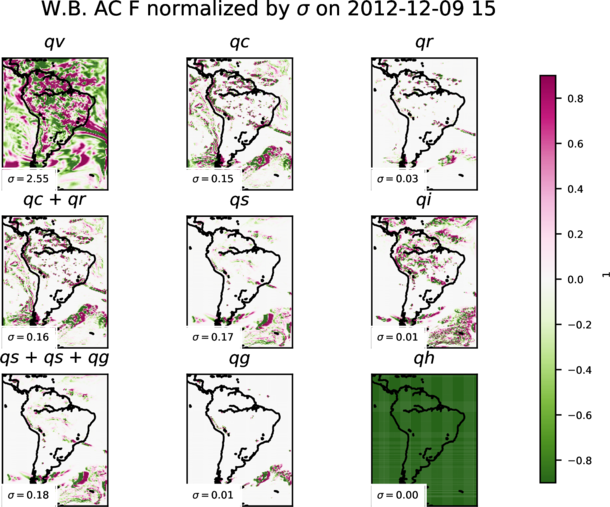
Preliminary results for all water species are shown in figures 1 and 2. Water vapour exhibits the largest values in both total tendency and horizontal advection. Dynamics of the other water species seems to be highly correlated with the presence of a storm system (lower right corner in the maps) or due to orthographic influences (existence of Andes range can be inferred).

Figure 1: Normalized (with the spatial standard deviation of the mapped values, σ) water budget 3h-accumulated vertically integrated total tendency `PW' at a given time, for water vapour (qv, top left), cloud (qc, top middle), rain (qr, top right), water condensed species (qc + qr, middle left), snow (qs, middle middle), ice (qi, middle right), water solid species (qs + qi + qg, bottom left), graupel (qg, bottom middle), hail (qh, bottom right). Number on low left corner of the figure correspond to the standard deviation (σ in mm) value used for the normalization

Figure 2: As in 1, but for Water budget 3h-accumulated vertically integrated horizontal advection `F' at a given time

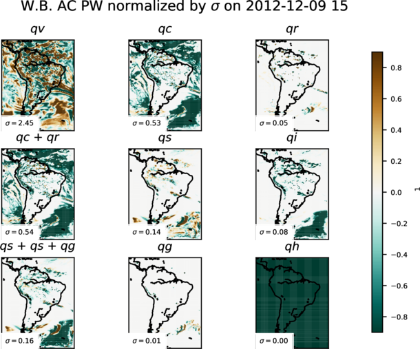
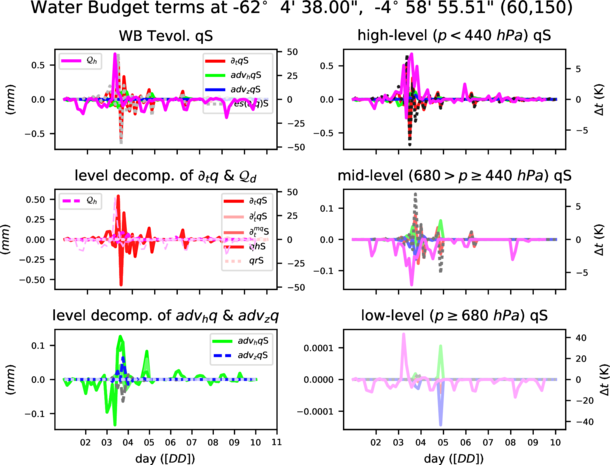
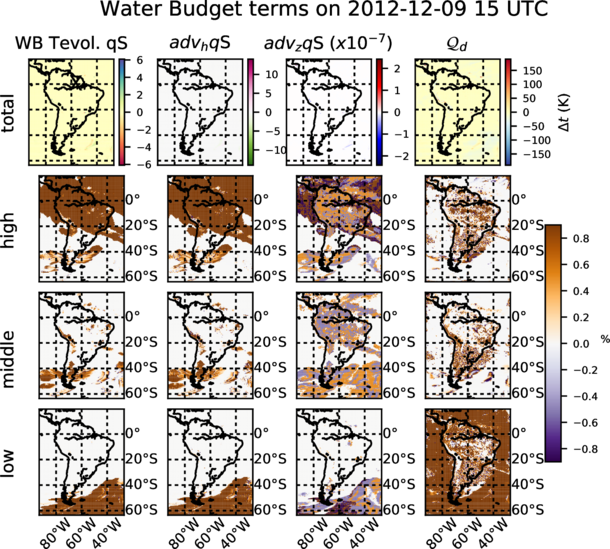
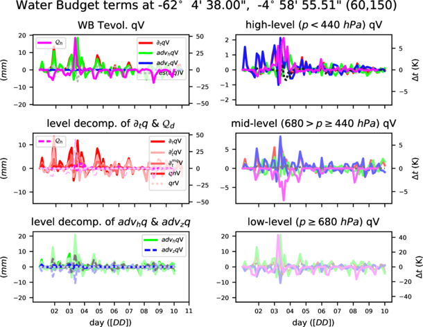
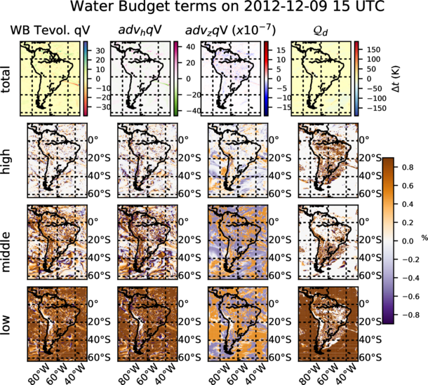
Figures from 3 to 6 show temporal evolution and accumulated maps at a given time for all the water budget terms, decomposed for vapour (qv) and snow (qs). Accumulated maps are grouped into vertical levels as it is done with the clouds: p ≥ 68000 P a, 40000 ≤ p < 68000 P a, p < 40000 P a. Largest amounts of the budget terms are mainly found in low (high) levels for water vapour (snow), temporal evolution at a given point show complexity of the water dynamics with the terms compensating each other. It is also shown how contribution to the total diabatic term is large at low levels over the ocean (showing the role of evaporation) and larger at high levels above the continent.

Figure 3: Water budget evolution at a given point for water vapour of vertically integrated water-budget terms: total tendency `PW' (∂<sub>t</sub>qv, red), horizontal advection `F' (adv_hqv, green), vertical advection `Z' (adv_zqv, green), residual PW-F-Z (res(∂_tqv), gray dashed) and diabatic heating from micro-physics (Q_d, pink) (top left), only high-level vertically integrated values (p < 440 hP a, top right), high/mid/low-level (degree of color intensity) decomposition of ∂_t qv (red) and Q_d (pink) and their respective residuals as dashed lines (middle left), only mid-level vertically integrated values (680 > p ≤ 440 hP a, middle right), high/mid/low-level (degree of color intensity) decomposition of adv_hqv (green) and adv_zqv (blue) and their respective residuals as dashed lines (bottom left) and only low-level vertically integrated values (p ≥ 680 hP a, bottom right)

Figure 4: Water vapour budget maps of each component and diabatic heating from micro-physics at a given time and the percentual contribution at each different vertically integrated layer respective the total. total tendency `PW' (∂<sub>t</sub>qv, first column), horizontal advection `F' (adv_hqv, second col), vertical advection `Z' (adv_zqv, third col.) and diabatic heating from micro-physics (Q_d, 4th col). Percentage contribution of high level (p < 440 hP a) integration to the total (second row), percentage for mid level (680 > p ≥ 440 hP a) integration to the total (third row) and percentage of low-level (p ≥ 680 hP a) integration (bottom row)

Figure 5: The same as in figure 3, but for snow

Figure 6: The same as in 4, bur for snow

fogvis: visibility inside fog

Fog is one of major causes of transportation disruption. The horizontal resolutions of state-of-the-art CORDEX activities like FPS_Alps (3 km) open the possibility to explore phenomena such as fog which was impossible to be analyzed in previous experiments. In order to be able to contribute in the analysis of fog phenomena, three different methods to calculate visibility have been introduced. Visibility is used to determine the presence of fog at a given moment. In order to provide a quantity with the density of the fog, only the visibility during a fog event is kept. The three methods are:

• K84 [visibility_diag = 1]: Visibility is computed using liquid water (QCLOUD) and ice (QICE) concentrations. Following (Bergot et al., 2007), fog appears when there are liquid and/or ice water species at the lowest model level present. Visibility is computed using equation 4 as in Kunkel (1984),

where QCLOUD: liquid water (cloud) mixing ratio (kgkg^-1), QICE: ice mixing ratio (kgkg^-1). Visibility values are in km

• RUC [visibility_diag = 2]: Visibility is computed using relative humidity (hur) as implemented in the RUC model (see equation 5 in Smirnova et al., 2000)

where hur: relative humidity (1, previously computed) and can be from the 2-m diagnostics or the first model layer. Visibility values are in km

• FRAM-L [visibility_diag = 3], (default): Visibility is computed using relative humidity (hur) after (see equation 6 in Gultepe and Milbrandt, 2010). In this work, a probabilistic approach is proposed to compute the visibility in three different bins: 95% , 50% and 5% of probability to get certain visibility (for rh > 30%). As a matter of compromise in the module, the calculation with the 50% of probability has been chosen as the preferred one. Therefore, this method provides the visibility that may occur with a 50% of probability.

where hur: relative humidity (1) and can be from 2-m diagnostics or first model layer. Visibility values are in km

Provided values of visibility during a fog event are: the minimum, maximum and mean values within output time steps (9freq) when fog occurred. Different choices are controlled throughout namelist variables: visibility_diag is isde to determine the method used to compute visibility, fogvars determines the source of the relative humidity to be used as input in the visibility method. User can choose to use the relative humidity from the first model layer (hur) fogvars=1 (default value) or from the 2-m diagnostics (hurs) fogvars=2. Some preliminary results of an extreme fog episode in central Argentina are provided in figure 7. Results strongly differ among fog implementations. The best agreement with a satellite visible channel picture for a given time of the event is obtained when the default setting is used (`FRAM-L' method with `hur' values as input).

Figure 7: On 2007 June 30th at 12, comparison of the different configurations of the diagnostics of the mean fog visibility (in 1 hour) to the satellite image from GOES-12 (top left) at the same time in the visible channel (courtesy of NOAA-CLASS), default vis3vars1 (fogvisibility=3, fogvars=1; top middle), vis3vars2 (top right), vis1vars1 (bottom left), vis2vars1 (bottom middle) and vis2vars2 (bottom right)

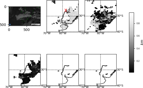
It is known that certain methods for calculating visibility relay on numerical adjustments on certain observational data taken under certain circumstances and at specific places (e.g.: for FRAM-L adjusted values come from observations from a Canadian airport). It would be desirable to provide a more generic "all places/purposes" approach (if possible). It is recommended to take this variable with a certain care.

tfog: time of presence of fog

Fog can be diagnosed when the visibility is lower than 1 km (WMO, 2010b). tfog accounts for the period during which the grid point has visibility lower than 1 km during 9freq (see equation 7)

where vis: visibility (km) below 1 km. δt: model time step (s)

References

• Bergot, T., Terradellas, E., Cuxart, J., Mira, A., Liechti, O., Mueller, M., and Nielsen, N. W. (2007). Intercomparison of single-column numerical models for the prediction of radiation fog. Journal of Applied Meteorology and Climatology, 46(4):504–521.
• Brasseur, O. (2001). Development and application of a physical approach to estimating wind gusts. Monthly Weather Review, 129(1):5–25.
• Fita, L., Fernández, J., and García-Díez, M. (2010). Clwrf: Wrf modifications for regional climate simulation under future scenarios. Proceedings of 11th WRF Users' Workshop.
• Fita, L. and Flaounas, E. (2018). Medicanes as subtropical cyclones: the december 2005 case from the perspective of surface pressure tendency diagnostics and atmospheric water budget. Q. J. Royal Met. Soc., doi: 10.1002/qj.3273
• García-Díez, M., Fernández, J., Fita, L., and Yagüe, C. (2013). Seasonal dependence of wrf model biases and sensitivity to pbl schemes over europe. Q. J. of Roy. Met. Soc., 139:501–514.
• Garratt, J. (1992). The Atmospheric Boundary Layer. Cambridge Univ. Press, Cambridge, U.K.
• Hourdin, F., Musat, I., Bony, S., Braconnot, P., Codron, F., Dufresne, J.-L., Fairhead, L., Filiberti, M.-A., Friedlingstein, P., Grandpeix, J.-Y., Krinner, G., LeVan, P., Li, Z.-X., and Lott, F. (2006). The LMDZ4 general circulation model: climate performance and sensitivity to parametrized physics with emphasis on tropical convection. Clim. Dyn., 27(7-8):787–813.
• Huang, H.-L., Yang, M.-J., and Sui, C.-H. (2014). Water budget and precipitation efficiency of typhoon Morakot (2009). J. Atmos. Sci., 71:112–129.
• Jourdier, B. (2015). Ressource éolienne en france métropolitaine : méthodes dâĂŹévaluation du potentiel, variabilité et tendances. Climatologie: École Doctorale Polytechnique, 2015. Français. ph:+33 01238226, pages 1–229.
• Kunkel, B. A. (1984). Parameterization of droplet terminal velocity and extinction coefficient in fog models. Journal of Climate and Applied Meteorology, 23(1):34–41.
• Monteith, J. L. (1965). Evaporation and environment. the state and movement of water in living organisms. 19th Symp. Soc. Exp. Biol, pages 205–234.
• Nielsen-Gammon, J. W., Powell, C. L., Mahoney, M. J., Angevine, W. M., Senff, C., White, A., Berkowitz, C., Doran, C., and Knupp, K. (2008). Multisensor estimation of mixing heights over a coastal city. Journal of Applied Meteorology and Climatology, 47(1):27–43.
• Skamarock, W. C., Klemp, J. B., Dudhia, J., Gill, D. O., Duda, D. M. B. M. G., Huang, X.-Y., Wang, W., and Powers, J. G. (2008). A description of the advanced research wrf version 3. NCAR TECHNICAL NOTE, 475:NCAR/TNÂŋ475+STR.
• Smirnova, T. G., Benjamin, S. G., and Brown, J. M. (2000). Case study verification of ruc/maps fog and visibility forecasts. Preprints, 9 th Conference on Aviation, Range, and Aerospace Meteorlogy, AMS, Orlando, FL, Sep. 2000, 2.3:6.
• WMO (2010). Guide to meteorological instruments and methods of observation. Weather - Climate - Weather, pages

1–176.

• Yang, M. J., Braun, S. A., and Chen, D.-S. (2011). Water budget of typhoon nari (2001). Mon. Wather Rev., 139:3809–3828.

Back to the main page CDXWRF